머신러닝(Machine Learning, ML)
- 데이터 수집과 처리 기술의 발전으로 대용량 데이터의 패턴을 인식하고 이를 바탕으로 예측, 분류하는 방법론
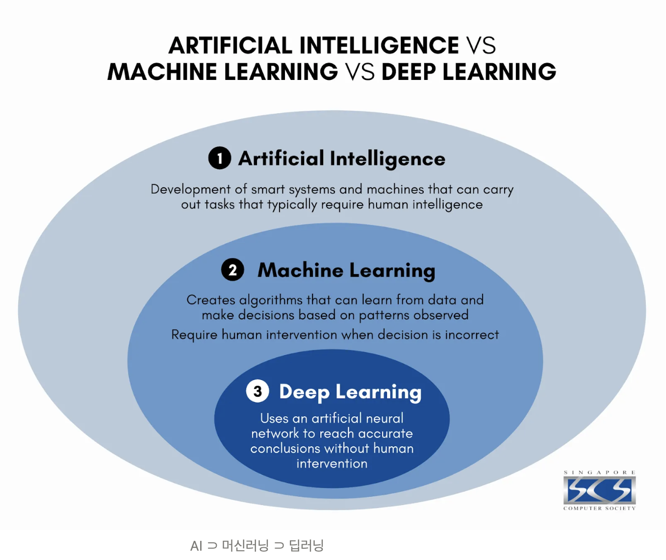
- AI: 인간의 지능을 요구하는 업무를 수행하기 위한 시스템
- Machine Learning: 관측된 패턴을 기반으로 의사 결정을 하기 위한 알고리즘
- Deep Learning: 인공신경망을 이용한 머신러닝
종류
- 지도 학습(Supervised Learning) : 문제와 정답을 모두 알려주고 공부시키는 방법, 예측&분류
- 비지도 학습(Unsupervised Learning) : 답을 가르쳐주지 않고 공부시키는 방법, 연관 규칙&군집
- 강화 학습(Reinforcement Learning) : 보상을 통해 상은 최대화, 벌은 최소화하는 방향으로 행위를 강화하는 학습
회귀분석 (숫자를 맞추는 것)
선형회귀
개념
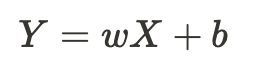
- Y : 종속 변수, 결과 변수
- X : 독립 변수, 원인 변수, 설명 변수
- : 가중치
- b : 편향(Bias)
- 장점 : 직관적이며 이해하기 쉽고 X-Y 관계를 정량화 할 수 있으며, 모델이 빠르게 학습됨(가중치 계산이 빠름)
- 단점 : X-Y간의 선형성 가정이 필요하며 평가지표에 평균을 포함하므로 이상치에 민감함, 범주형 변수를 인코딩 시 정보 손실이 일어남
- 패키지 : sklearn.linear_model.LinearRegression
평가 지표
MSE(Mean Squared Erorr)
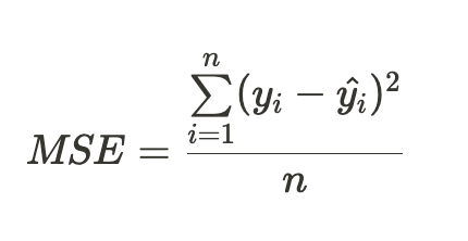
- 에러(실제 데이터 - 추정 데이터)의 값을 제곱하여 양수를 만들어 모두 더한 후 데이터만큼 나눈 것
- 숫자 예측 문제는 모델은 MSE 지표를 최소화하는 방향으로 진행하고 평가함
RMSE
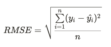
- MSE에 Root를 씌워 제곱 된 단위를 다시 맞춤
MAE
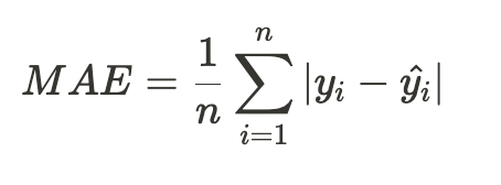
- 절대 값을 이용하여 오차 계산
R Square
- 선형회귀만의 평가 지표
- 전체 모형에서 회귀선으로 설명할 수 있는 정도
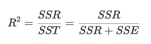
-SST : total sum of squares
-SSE : error sum of squares
-SSR : regression sum of squares
적용
- 단순선형회귀
# 라이브러리 import
import sklearn
import numpy as np
import pandas as pd
import matplotlib.pyplot as plt
import seaborn as sns

# 산점도 먼저 확인
sns.scatterplot(data = body_df, x = 'weight', y = 'height')
plt.title('Weight vs Height')
plt.xlabel('Weight(kg)')
plt.ylabel('Height(cm)')
plt.show()

# 선형회귀 적합 시 훈련
from sklearn.linear_model import LinearRegression
model_lr = LinearRegression()
type(model_lr)

# DataFrame[]: Series(데이터 프레임의 컬럼)
# DataFrame[[]]: DataFrame
X = body_df[['weight']]
y = body_df[['height']]

# 데이터 훈련
model_lr.fit(X = X, y = y)

# 가중치(w1)
w1 = model_lr.coef_[0][0]
# 편향(bias, w0)
w0 = model_lr.intercept_[0]

# 공식 적용
print('y = {}x + {}'.format(w1.round(2),w0.round(2)))

# 함수 import (서브 모듈이라 따로 가져와야 함)
from sklearn.metrics import mean_squared_error, r2_score

# 예측값 생성(평가함수는 실제 true, 예측값 pred)
y_true = body_df['height']
y_pred = model_lr.predict(body_df[['weight']])

# 에러 계산 = MSE
mean_squared_error(y_true, y_pred)

# r square 분석 = 분야의 적정 기중치가 있고, 높을수록 연관이 있음
r2_score(y_true, y_pred)

# 시각화 - 산점도 그래프에 선형식 추가
sns.scatterplot(data = body_df, x = 'weight', y = 'height')
sns.lineplot(data = body_df, x = 'weight', y = 'pred', color = 'red')
심화
- 범주형 데이터에 적용 & 다중선형회귀
# seaborn 라이브러리를 통해 데이터셋 가져오기
tips_df = sns.load_dataset('tips')

# 범주형 데이터 인코딩(Female 0, Male 1)
def get_sex(x):
    if x == 'Female':
        return 0
    else:
        return 1

# apply method를 활용하여 모든 행에 함수 적용
tips_df['sex_en'] = tips_df['sex'].apply(get_sex)

# 모델설계도 가져오기
model_lr2 = LinearRegression()
X = tips_df[['total_bill','sex_en']]
y = tips_df[['tip']]

#학습
model_lr2.fit(X,y)

#예측
y_true_tip = tips_df['tip']
y_pred_tip = model_lr2.predict(X)

# 평가
mean_squared_error(y_true_tip, y_pred_tip) # MSE
r2_score(y_true_tip, y_pred_tip)
분류분석 (카테고리를 맞추는 것)
로지스틱회귀
개념
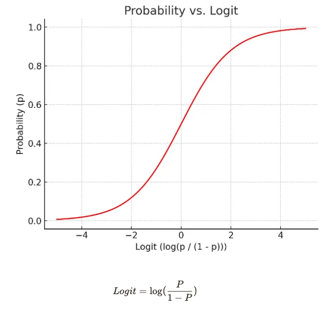
- 선형회귀에서 종속 변수(Y)가 특정 값이 아닌 특정 값이 될 확률
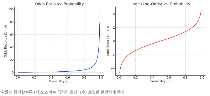
- 오즈비(odds ratio) : 실패확률 대비 성공확률
- 로짓(logit) : 확률은 0과 1 사이인데, 확률이 증가할수록 오즈비가 급증해 선형성을 따르지 않기 때문에 로그를 씌워 보정한 것
평가 지표
혼돈 행렬(confusion Matrix)
- 실제 값과 예측 값에 대한 모든 경의 수를 표현하는 2x2 행렬
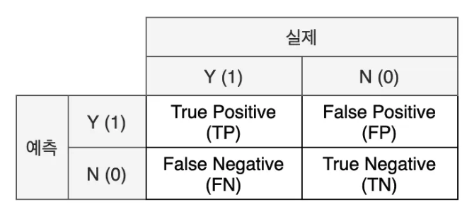
- 실제와 예측이 같으면 True 다르면 False
- 예측을 양성으로 했으면 Positive 음성이면 Negative
- 지표
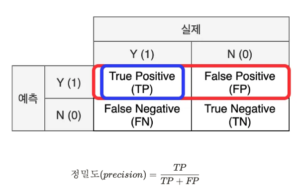
-정밀도(Precision) : 모델이 양성(1)로 예측한 결과 중 실제 양성의 비율, 모델 관점
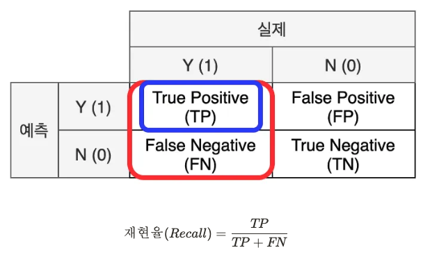
-재현율(Recall) : 실제 값이 양성인 데이터 중 모델이 양성으로 예측한 비율, 데이터 관점
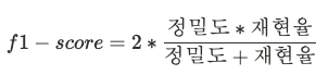
-f1 Score : 정밀도와 재현율의 조화 평균
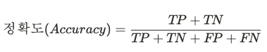
-정확도(Accuracy) : 맞춘 정답을 전체 데이터 개수로 나누는 것
적용
- 함수
속성
-classes_: 클래스(Y)의 종류
-n_features_in_: 들어간 독립변수(X) 개수
-feature_names_in_: 들어간 독립변수(X)의 이름
-coef_: 가중치
-intercept_: 바이어스
메소드
-fit: 데이터 학습
-predict: 데이터 예측
-predict_proba: 데이터가 Y = 1일 확률을 예측
-sklearn.metrics.accuracy: 정확도
-sklearn.metrics.f1_socre: f1_score
- 1차 모델(X가 하나)
# 라이브러리 import
import pandas as pd
import numpy as np
import matplotlib.pyplot as plt
import seaborn as sns
from sklearn.linear_model import LogisticRegression

# 변수 선언 - X는 수치형이 좋음
X_1 = titaninc_df[['Fare']]
y_true = titaninc_df[['Survived']]

# 각종 그래프 확인
sns.scatterplot(titaninc_df, x = 'Fare',y = 'Survived') # 산점도
sns.histplot(titaninc_df, x = 'Fare') # 히트맵
titaninc_df.describe() # 수치형 데이터 확인

# 모델설계도 가져오기
model_lor = LogisticRegression()
model_lor.fit(X_1, y_true)

# 모델 각종 수치 확인 함수
def get_att(x):
    print('클래스 종류', x.classes_)
    print('독립변수 갯수', x.n_features_in_)
    print('들어간 독립변수(x)의 이름',x.feature_names_in_)
    print('가중치',x.coef_)
    print('바이어스', x.intercept_)

get_att(model_lor)

# 평가 함수
from sklearn.metrics import accuracy_score, f1_score
def get_metrics(true, pred):
    print('정확도', accuracy_score(true, pred))
    print('f1-score', f1_score(true, pred))

# 예측
y_pred_1 = model_lor.predict(X_1)

# 평가
get_metrics(y_true, y_pred_1)- 다중 로지스틱회귀(X 2개 이상)
# 범수형 변수 인코딩
def get_sex(x):
    if x == 'female':
        return 0
    else:
        return 1
titaninc_df['Sex_en'] = titaninc_df['Sex'].apply(get_sex)

# 변수 선언
X_2 = titaninc_df[['Pclass','Sex_en','Fare']]
y_true = titaninc_df[['Survived']]

# 모델 가져오기
model_lor_2 = LogisticRegression()

# 학습
model_lor_2.fit(X_2,y_true)

# 예측
y_pred_2 = model_lor_2.predict(X_2)

# 평가
get_metrics(y_true, y_pred_2)

# 각 데이터별 Y=1인 확률
model_lor_2.predict_proba(X_2)
👋🏻