환경설정(colab)
from google.colab import drive
drive.mount('/content/gdrive')
폴더 경로 설정
workspace_path = '/content/gdrive/경로'필요 패키지 로드
import cv2
from PIL import Image
from urllib import request
import io
import numpy as np
import matplotlib.pyplot as plt
import torch
import torchvision
import os
image_list = []
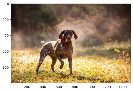
url_1 = "https://www.southernliving.com/thmb/9E2guP65DZP_ZnUP13pcVG8Sfmc=/1500x0/filters:no_upscale():max_bytes(150000):strip_icc()/GettyImages-1285438779-2000-9ea25aa777df42e6a046b10d52b286b7.jpg"
res_1 = request.urlopen(url_1).read()
img_1 = Image.open(io.BytesIO(res_1))
image_list.append(img_1)
img_array_1 = np.array(img_1)
plt.imshow(img_array_1)
plt.show()
###################################################################################################################
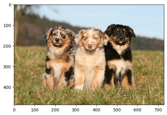
url_2 = "https://www.akc.org/wp-content/uploads/2018/05/Three-Australian-Shepherd-puppies-sitting-in-a-field.jpg"
res_2 = request.urlopen(url_2).read()
img_2 = Image.open(io.BytesIO(res_2))
image_list.append(img_2)
img_array_2 = np.array(img_2)
plt.imshow(img_array_2)
plt.show()
###################################################################################################################
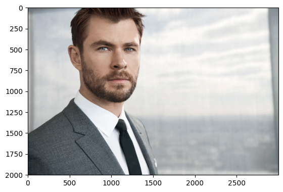
url_3 = "https://images.lifestyleasia.com/wp-content/uploads/2019/10/18094733/1128_01_2610.jpg"
res_3 = request.urlopen(url_3).read()
img_3 = Image.open(io.BytesIO(res_3))
image_list.append(img_3)
img_array_3 = np.array(img_3)
plt.imshow(img_array_3)
plt.show()
print(len(image_list))
model = torch.hub.load('pytorch/vision:v0.10.0', 'fcn_resnet50', pretrained=True) ## 온라인 상이나 로컬상의 프리트레이닝 셋을 불러옴
model.eval() ## 검증모드로 변경 ## 기울기의 특정 변화는 없다#결과 :
3
Segmentation 1
from PIL import Image
from torchvision import transforms
import matplotlib.pyplot as plt
import random
from glob import glob
import numpy as np
# image_shape : H W C (0, 1, 2) -> (permute(2, 1, 0)) -> C H W
# model_input : B C H W
# permute, traspose(회전)
preprocess = transforms.Compose([
transforms.ToTensor(),
transforms.Normalize(mean=[0.485, 0.456, 0.406], std=[0.229, 0.224, 0.225]),
])
# image_list = sorted(glob(os.path.join(workspace_path, 'PASCAL_VOC/VOCdevkit/VOC2012/JPEGImages')+'/*.jpg'))
print(len(image_list))
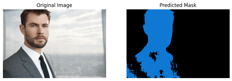
for idx in range(3) : ## idx = 0, 1, 2
# input_image = Image.open(image_list[random.randint(0,len(image_list))])
input_image = image_list[idx]
input_image = input_image.convert("RGB") ## BGR타입일 경우 RGB로 변경
input_tensor = preprocess(input_image)
input_batch = input_tensor.unsqueeze(0) # 모델에서 요구되는 미니배치 생성
## unsqueeze : 채널의 축을 생성
## [C H W] -> [B C H W]
## input_batch = input_tensor.unsqueeze(0) 에서 unsqueeze를 빼고 실행하면 아래와 같이 변경
## [C H W] -> [ H W]
input_batch = input_batch.to('cuda') ## GPU에서 처리를 하게 해줌
model.to('cuda') ## GPU에서 처리를 하게 해줌
with torch.no_grad(): ## 검증 단계에서는 기울기가 필요없기에 실행
output = model(input_batch)['out'][0]
#torch.argmax() -> 340x1440 [h, w]
print(output.shape) ## 결과 : torch.Size([21, 1000, 1500]) ## voc21 : 클래스 개수
output_predictions = output.argmax(0) ## 여러 개의 레이어 ## 0번 채널에서 가장 큰 숫자
print(torch.unique(output_predictions)) ## 결과 예시 : tensor([ 0, 3, 8, 12, 13, 15, 17], device='cuda:0') 숫자들은 각각 클래스를 의미함 ## 0은 배경, 8은 고양이...
palette = torch.tensor([2 ** 25 - 1, 2 ** 15 - 1, 2 ** 21 - 1]) ## 색깔 표시 ## 각 클래스 색깔 정해줌
colors = torch.as_tensor([i for i in range(21)])[:, None] * palette ## for문을 돌리면서 tensor로 변경 후 palette를 곱해줌 ## -> [0,122,355] 처럼 색깔 정보가 나옴
colors = (colors % 255).numpy().astype("uint8")
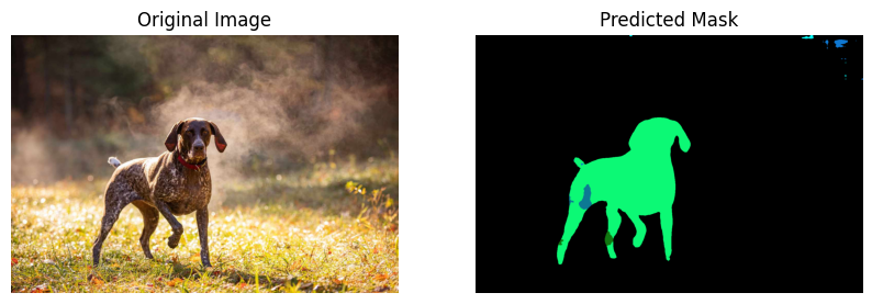
# 21개 클래스의 Semantic Segmentation Prediction을 그림으로 표시
mask = Image.fromarray(output_predictions.byte().cpu().numpy()).resize(input_image.size) ## byte로 바꾸고 cpu로 바꾸고 numpy로 바꾸고 사이즈를 맞춰줌
mask.putpalette(colors) ## 색상 입히기
plt.figure(figsize=(10, 5)) ## plt 사이즈 정의
plt.subplot(1, 2, 1)
plt.imshow(input_image)
plt.title('Original Image')
plt.axis('off')
plt.subplot(1, 2, 2)
plt.imshow(mask)
plt.title('Predicted Mask')
plt.axis('off')
plt.show()#결과 :
3
torch.Size([21, 1000, 1500])
tensor([ 0, 3, 8, 12, 13, 15, 17], device='cuda:0')
torch.Size([21, 486, 729])
tensor([ 0, 8, 12], device='cuda:0')
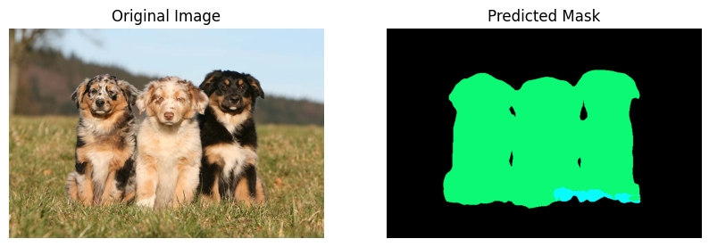
torch.Size([21, 2002, 3000])
tensor([ 0, 7, 11, 15], device='cuda:0')
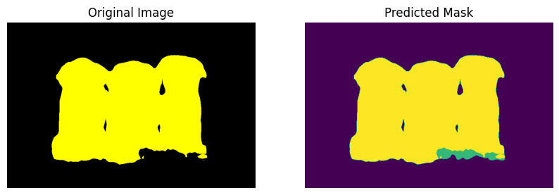
Segmentation 2
preprocess = transforms.Compose([
        transforms.ToTensor(),
        transforms.Normalize(mean=[0.485, 0.456, 0.406], std=[0.229, 0.224, 0.225]),
    ])


input_image = image_list[1]
input_image = input_image.convert("RGB")  ## BGR타입일 경우 RGB로 변경

input_tensor = preprocess(input_image)
input_batch = input_tensor.unsqueeze(0) # 모델에서 요구되는 미니배치 생성

input_batch = input_batch.to('cuda')  ## GPU에서 처리를 하게 해줌
model.to('cuda') ## GPU에서 처리를 하게 해줌


with torch.no_grad():  ## 검증 단계에서는 기울기가 필요없기에 실행
  output = model(input_batch)['out'][0]

output_predictions = output.argmax(0)  ## 여러 개의 레이어  ## 0번 채널에서 가장 큰 숫자
print(torch.unique(output_predictions))  ## 결과 예시 : tensor([ 0,  3,  8, 12, 13, 15, 17], device='cuda:0')  숫자들은 각각 클래스를 의미함 ## 0은 배경, 8은 고양이...

palette = torch.tensor([2 ** 25 - 1, 2 ** 15 - 1, 2 ** 21 - 1])  ## 색깔 표시  ## 각 클래스 색깔 정해줌
colors = torch.as_tensor([i for i in range(21)])[:, None] * palette  ## for문을 돌리면서 tensor로 변경 후 palette를 곱해줌 ## -> [0,122,355] 처럼 색깔 정보가 나옴
colors = (colors % 255).numpy().astype("uint8")

# 21개 클래스의 Semantic Segmentation Prediction을 그림으로 표시
mask = Image.fromarray(output_predictions.byte().cpu().numpy()).resize(input_image.size) ## byte로 바꾸고 cpu로 바꾸고 numpy로 바꾸고 사이즈를 맞춰줌
mask.putpalette(colors) ## 색상 입히기
plt.figure(figsize=(10, 5)) ## plt 사이즈 정의

mask = np.array(mask)
print(mask.shape)
print(np.unique(mask))

print(np.where(mask == 12)[0].shape, np.where(mask == 12)[1].shape)
 ## 점의 좌료 : (x, y)

input_array = np.array(input_image)
print(input_array[np.where(mask == 8)]) ## 결과 예시 :

input_array[np.where(mask == 12)] = (255, 255, 0) ## 강아지는 노란색으로
input_array[np.where(mask != 12)] = (0, 0, 0)  ## 그 이외에는 검은색으로

input_image = Image.fromarray(input_array)

plt.subplot(1, 2, 1)
plt.imshow(input_image)
plt.title('Original Image')
plt.axis('off')

plt.subplot(1, 2, 2)
plt.imshow(mask)
plt.title('Predicted Mask')
plt.axis('off')
plt.show()
#결과 :
tensor([ 0, 8, 12], device='cuda:0')
(486, 729)
0 8 12 (117837,)
[[249 202 158][253 208 166]
[252 206 156]
...
[143 114 58][149 109 57]
[149 102 48]]

공부 기록