데브코스 자율주행 최종 프로젝트 - 16주차 금요일 TIL

오늘 한 일

• LiDAR Data 시각화
• LiDAR 3D Point Cloud 2D projection
• 2D projection된 LiDAR Data 이미지에 씌우기

결과

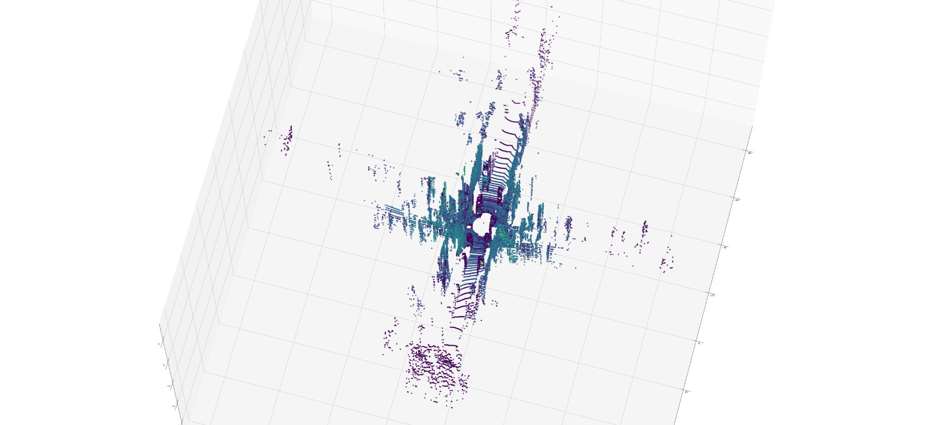
LiDAR 3D Point cloud 시각화

: 기존 matlab 코드를 python으로 수정해 시각화

import numpy as np
import matplotlib.pyplot as plt
from mpl_toolkits.mplot3d import Axes3D

# 파일 읽기
with open('/workspace/KITTI/KITTI_road/data_road_velodyne/training/velodyne/uu_000024.bin', 'rb') as f:
    data = np.fromfile(f, dtype=np.float32)

# 데이터 재구성
data = data.reshape(-1, 4)

# 시각화
fig = plt.figure(figsize = (80, 60))
ax = fig.add_subplot(111, projection='3d')
ax.scatter(data[:, 0], data[:, 1], data[:, 2], c=data[:, 3], cmap='viridis')  # x, y, z, color, colormap
ax.view_init(70, 15) # change viewpoint
plt.savefig('./output.jpg')

• LiDAR 3D Point cloud 시각화 결과
  

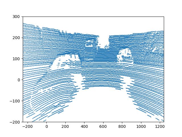
LiDAR Point cloud 2D projection 및 image data와 병합

: 기존 matlab 코드를 python으로 수정해 시각화

import numpy as np
import cv2
import matplotlib.pyplot as plt
from mpl_toolkits.mplot3d import Axes3D
import open3d as o3d

# read calibration file and parse the matrices
filepath = "/workspace/KITTI/KITTI_road/data_road/training/"

with open(filepath + 'calib/uu_000024.txt', 'r') as fid:
    lines = fid.readlines()
    P0 = np.fromstring(lines[0].split(': ')[1], dtype=float, sep=' ')
    P1 = np.fromstring(lines[1].split(': ')[1], dtype=float, sep=' ')
    P2 = np.fromstring(lines[2].split(': ')[1], dtype=float, sep=' ')
    P3 = np.fromstring(lines[3].split(': ')[1], dtype=float, sep=' ')
    R0_rect = np.fromstring(lines[4].split(': ')[1], dtype=float, sep=' ')
    Tr_velo_to_cam = np.fromstring(lines[5].split(': ')[1], dtype=float, sep=' ')
    Tr_imu_to_velo = np.fromstring(lines[6].split(': ')[1], dtype=float, sep=' ')
    Tr_cam_to_road = np.fromstring(lines[7].split(': ')[1], dtype=float, sep=' ')

Tr = np.vstack((np.reshape(Tr_velo_to_cam, (3, 4)), [0, 0, 0, 1]))
R0 = np.eye(4)
R0[:3, :3] = np.reshape(R0_rect, (3, 3))
P = np.reshape(P2, (3, 4))

# read image
img = cv2.imread(filepath + 'image_2/uu_000024.png')
img_mapped = img.copy()
# plt.imshow(img)
# plt.show()

# read LiDAR data
with open(filepath + 'velodyne/uu_000024.bin', 'rb') as fid:
    data = np.fromfile(fid, dtype=np.float32)

data = np.reshape(data, (-1, 4))
fig = plt.figure()
ax = fig.add_subplot(111, projection='3d')
ax.scatter(data[:, 0], data[:, 1], data[:, 2], c=data[:, 3], cmap='gray')
# plt.show()

# mapping to image
XYZ1 = np.vstack((data[:, :3].T, np.ones(data.shape[0]))) # world coordinate
xy1 = np.dot(P, np.dot(R0, np.dot(Tr, XYZ1))) # image coordinate

s = xy1[2, :]
x = xy1[0, :] / s
y = xy1[1, :] / s
k = np.where(s < 0)
plt.figure()
plt.plot(x[k], y[k], '.', markersize = 3)
plt.gca().invert_yaxis()
plt.xlim(0, img.shape[1])
plt.ylim(0, img.shape[0])
# plt.savefig('./output/lidar_image.jpg')

# mapping to image for marking valid LiDAR points
img_h, img_w, _ = img.shape
for i in range(len(s)):
    ix = int(x[i] + 0.5)
    iy = int(y[i] + 0.5)
    if s[i] <= 0 or ix <= 0 or ix >= img_w or iy <= 0 or iy >= img_h:
        continue
    img_mapped[iy, ix] = [0, 255, 0]

# cv2.imshow('Mapped Image', img_mapped)
# cv2.waitKey(0)
# cv2.destroyAllWindows()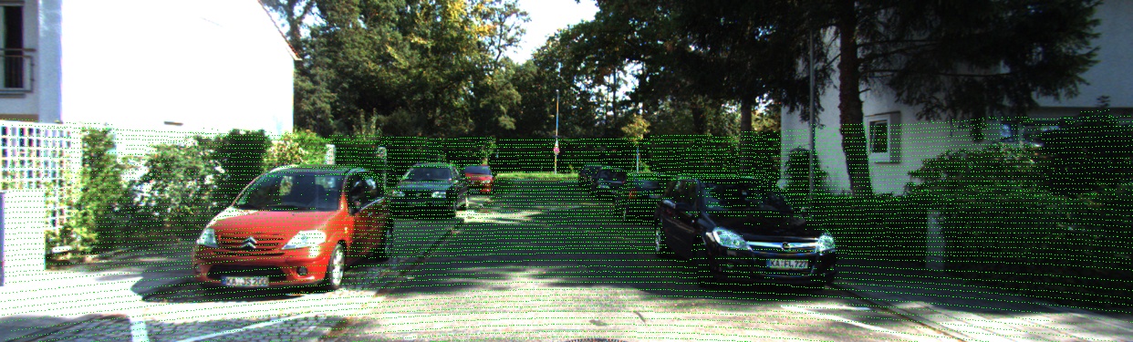
cv2.imwrite('./output/img_mapped.jpg', img_mapped)

• LiDAR Point cloud 2D projection 결과
  
  
• 2D projection된 LiDAR Data 이미지 병합 결과
  

[참고 사이트] : https://darkpgmr.tistory.com/190