Data Preparation
import pandas as pd
import numpy as np
import seaborn as sns
import matplotlib.pyplot as plt
from sklearn.datasets import load_breast_cancer
from sklearn.model_selection import train_test_split
from sklearn.preprocessing import StandardScaler
import torch
import torch.nn as nn
import torch.optim as optim
from torch.utils.data import DataLoader, TensorDataset
import torchmetrics
from sklearn.metrics import accuracy_score, precision_score, recall_score, f1_score, roc_auc_score, confusion_matrix
Load Data
data =load_breast_cancer()
df = pd.DataFrame(data.data, columns=data.feature_names)
df['target'] = data.target
df.head()
Explanatory Data Analysis
df.isnull().sum()mean radius 0
mean texture 0
mean perimeter 0
mean area 0
mean smoothness 0
mean compactness 0
mean concavity 0
mean concave points 0
mean symmetry 0
mean fractal dimension 0
radius error 0
texture error 0
perimeter error 0
area error 0
smoothness error 0
compactness error 0
concavity error 0
concave points error 0
symmetry error 0
fractal dimension error 0
worst radius 0
worst texture 0
worst perimeter 0
worst area 0
worst smoothness 0
worst compactness 0
worst concavity 0
worst concave points 0
worst symmetry 0
worst fractal dimension 0
target 0
dtype: int64df.describe()sns.countplot(x=df["target"])
plt.title("Distribution of Target Variable")
plt.show()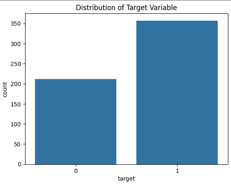
df.iloc[:,:12].hist(figsize=(12,8), bins=30)
plt.tight_layout()
plt.show()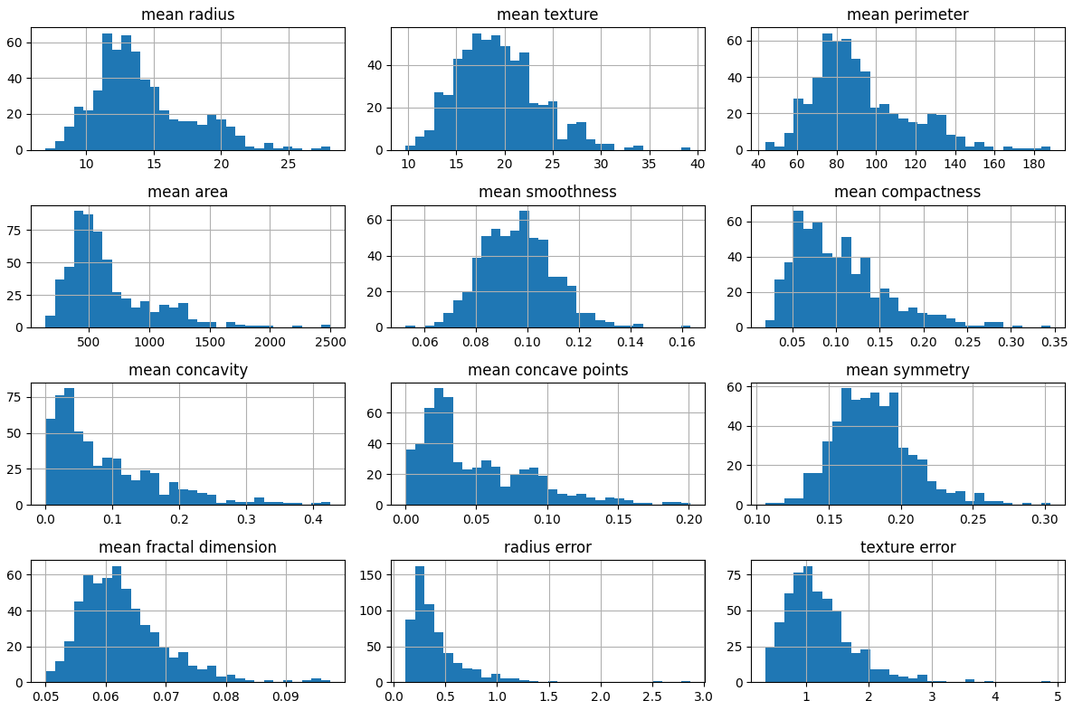
plt.figure(figsize=(12,8))
sns.heatmap(df.corr(), cmap="coolwarm", annot=False, fmt='.2f')
plt.title("Feature Correlation Heatmap")
plt.show()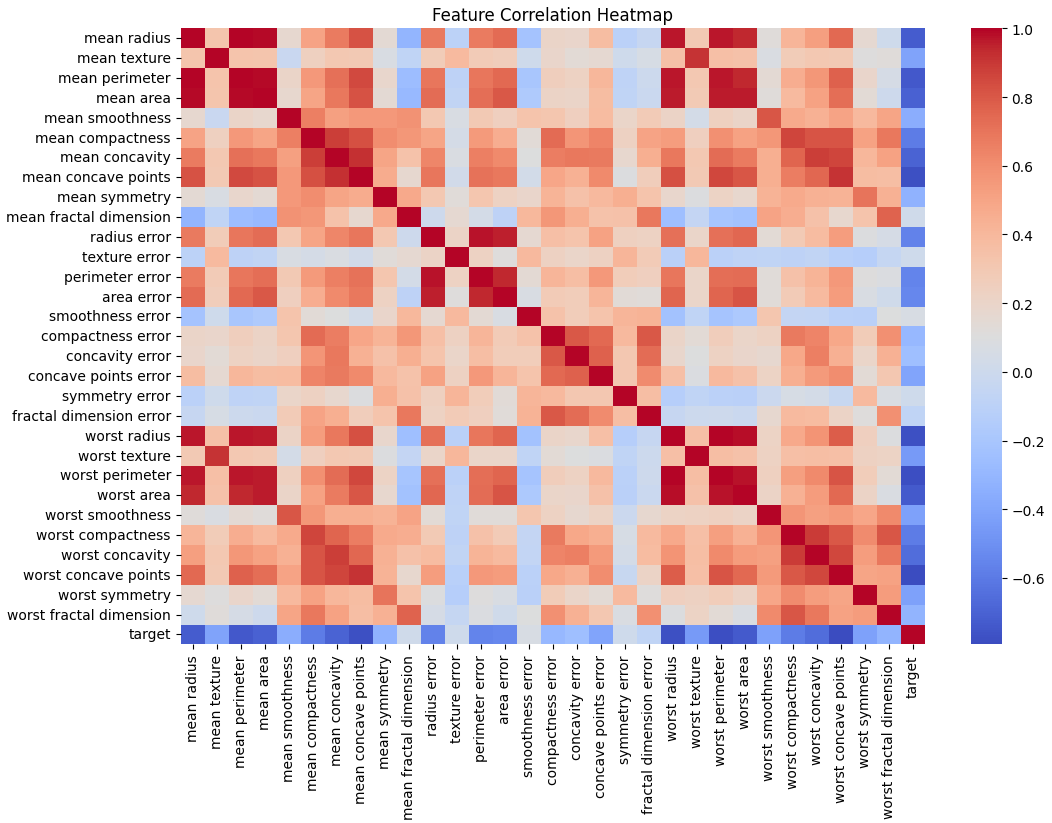
sns.pairplot(df.iloc[:,-5:], hue="target", diag_kind="kde")
plt.show()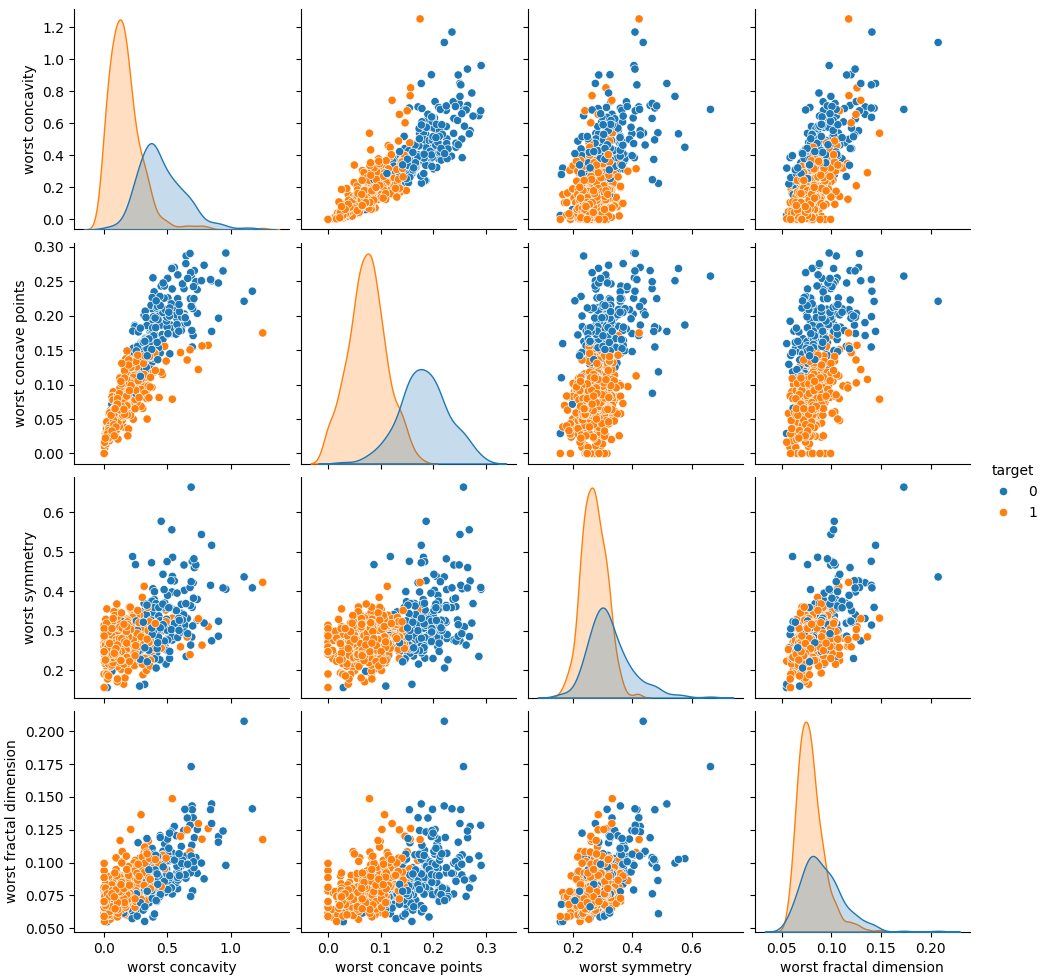
Feature Preprocessing
Separate X and Y
# Separate features and target variable
X = df.drop(columns = "target")
y = df['target']
Standardize the features
from sklearn.preprocessing import StandardScaler

# Standardize the features making the means 0 and standard deviations 1
scaler = StandardScaler()
X_scaled = scaler.fit_transform(X)

# Convert back to a Pandas Dataframe
X_scaled_df = pd.DataFrame(X_scaled, columns=X.columns)

X_scaled_df.describe()
Find Highly Correlated Features
# Compute correlation matrix
correlation_matrix = df.corr().abs()

# Select upper triangle of correlation matrix
upper= correlation_matrix.where(np.triu(np.ones(correlation_matrix.shape), k=1).astype(bool))

# Find features with correlation > 0.9
highly_correlated_features = [column for column in upper.columns if any(upper[column] > 0.9)]
print("Highly correlated features to drop: ", highly_correlated_features)
Highly correlated features to drop: ['mean perimeter', 'mean area', 'mean concave points', 'perimeter error', 'area error', 'worst radius', 'worst texture', 'worst perimeter', 'worst area', 'worst concave points']Drop highly correlated features
# Drop highly correlated features
X_selected = X_scaled_df
X_selected = X_scaled_df.drop(columns=highly_correlated_features)
Train-Test Split
Split data into train and test
# Split data into train (80%) and test (20%)
X_train, X_test, y_train, y_test = train_test_split(X_selected, y, test_size=0.2, random_state=42)
Convert data into PyTorch tensors
# Convert to PyTorch tensors
X_train = torch.tensor(X_train.values, dtype=torch.float32)
X_test = torch.tensor(X_test.values, dtype=torch.float32)
y_train = torch.tensor(y_train.values.reshape(-1,1), dtype = torch.float32)
y_test = torch.tensor(y_test.values.reshape(-1,1), dtype=torch.float32)

print("Training data shape: ", X_train.shape)
print("Testing data shape: ", X_test.shape)
Training data shape: torch.Size([455, 20])
Testing data shape: torch.Size([114, 20])Define Neural Network
You can use Sequential() for a simple model like this, but it is ultimately less customizable.
class BreastCancerClassifier(nn.Module):
    def __init__(self, input_dim):
        super(BreastCancerClassifier, self).__init__()
        print("Input Dim: ", input_dim)
        self.layer1 = nn.Linear(input_dim, 16)
        self.batchnorm1 = nn.BatchNorm1d(16, eps=1e-4, momentum=0.05, affine=True, track_running_stats=True)
        self.relu1 = nn.ReLU()
        self.layer2 = nn.Linear(16, 8)
        self.batchnorm2 = nn.BatchNorm1d(8, eps=1e-4, momentum=0.05, affine=True, track_running_stats=True)
        self.relu2 = nn.ReLU()
        self.layer3 = nn.Linear(8, 1)

        self.apply(self.initialize_weights)

    def initialize_weights(self, m):
        if isinstance(m, nn.Linear):
            if m.out_features == 1:
                nn.init.xavier_uniform_(m.weight) # Xavier for Sigmoid
            else:
                init.kaiming_uniform_(m.weight, nonlinearity="relu") # He for ReLU layers
            nn.init.zeros_(m.bias)

    def forward(self, x):
        # print(f"Input Shape: {x.shape}")
        x = self.relu1(self.layer1(x))
        x = self.batchnorm1(x)
        # print(f"After Layer 1: {x.shape}")
        x = self.relu2(self.layer2(x))
        x = self.batchnorm2(x)
        # print(f"After Layer 2: {x.shape}")
        x = self.layer3(x) # Return raw logits (No Sigmoid here)
        # print(f"Output Shape: {x.shape}")
        return x
Train the Model
input_dim = X_train.shape[1]
model = BreastCancerClassifier(input_dim)
device = "cuda" if torch.cuda.is_available() else "cpu"

model.to(device)
Input Dim: 20
BreastCancerClassifier(
(layer1): Linear(in_features=20, out_features=16, bias=True)
(batchnorm1): BatchNorm1d(16, eps=0.0001, momentum=0.05, affine=True, track_running_stats=True)
(relu1): ReLU()
(layer2): Linear(in_features=16, out_features=8, bias=True)
(batchnorm2): BatchNorm1d(8, eps=0.0001, momentum=0.05, affine=True, track_running_stats=True)
(relu2): ReLU()
(layer3): Linear(in_features=8, out_features=1, bias=True)
)Loss Function & Optimizer
from torch.optim.lr_scheduler import StepLR

loss_function = nn.BCEWithLogitsLoss() # Internally applies Sigmoid in a stable way
optimizer = optim.AdamW(model.parameters(), lr=0.01, betas=(0.9, 0.99), eps=1e-8) # Adam optimizer
scheduler = StepLR(optimizer, step_size=100, gamma=0.1)  # Decays LR every 100 epochs
batch_size = 32 # Adjust batch size as needed
train_dataset = TensorDataset(X_train, y_train)
train_loader = DataLoader(train_dataset, batch_size=batch_size, shuffle=True)epochs = 1000
loss_history = []
for epoch in range(epochs):
model.train()
epoch_loss = 0 # Reset epoch loss at the beginning of each epoch
for batch_X, batch_y in train_loader: # Iterate over mini-batches
batch_X, batch_y = batch_X.to(device), batch_y.to(device) # Move data to correct device
optimizer.zero_grad() # Reset gradients
outputs = model(batch_X) # Feedforward
loss = loss_function(outputs, batch_y) # Compute loss
loss.backward() # Compute gradients via backpropagation
optimizer.step() # Update weights
epoch_loss += loss.detach().item() # Accumuilate loss for logging (avoid extra computation)
loss_history.append(epoch_loss / len(train_loader)) # Store loss
scheduler.step() # Update learning rate
if (epoch+1) % 100 == 0:
print(f"Epoch [{epoch+1}/{epochs}], LR: {scheduler.get_last_lr()[0]:.6f}, Loss: {epoch_loss / len(train_loader):.4f}")Epoch [100/1000], LR: 0.001000, Loss: 0.0073
Epoch [200/1000], LR: 0.000100, Loss: 0.0062
Epoch [300/1000], LR: 0.000010, Loss: 0.0144
Epoch [400/1000], LR: 0.000001, Loss: 0.0021
Epoch [500/1000], LR: 0.000000, Loss: 0.0147
Epoch [600/1000], LR: 0.000000, Loss: 0.0014
Epoch [700/1000], LR: 0.000000, Loss: 0.0031
Epoch [800/1000], LR: 0.000000, Loss: 0.0784
Epoch [900/1000], LR: 0.000000, Loss: 0.0011
Epoch [1000/1000], LR: 0.000000, Loss: 0.0014# Plot loss history
plt.plot(range(epochs), loss_history, label="Training Loss")
plt.xlabel("Epoch")
plt.ylabel("Loss")
plt.legend()
plt.title("Training Loss Over Epochs")
plt.show()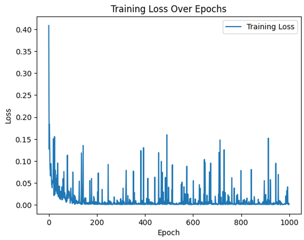
Model Evaluation
def evaluate_model(model, data_loader, dataset_name="Test", threshold=0.5):
    """Evaluates model performance using torchmetrics."""
    device = "cuda" if torch.cuda.is_available() else "cpu"
    model.eval()  # Set model to evaluation mode
    model.to(device)  # Move model to correct device

    # Define metrics
    accuracy = torchmetrics.Accuracy(task="binary").to(device)
    precision = torchmetrics.Precision(task="binary").to(device)
    recall = torchmetrics.Recall(task="binary").to(device)
    f1 = torchmetrics.F1Score(task="binary").to(device)
    roc_auc = torchmetrics.AUROC(task="binary").to(device)
    conf_matrix = torchmetrics.ConfusionMatrix(task="binary", num_classes=2).to(device)

    total_loss = 0  # Track test loss
    all_preds = []
    all_labels = []

    with torch.no_grad():
        for batch_X, batch_y in data_loader:
            batch_X, batch_y = batch_X.to(device), batch_y.to(device)

            logits = model(batch_X)  # Get raw logits
            probs = torch.sigmoid(logits)  # Convert logits to probabilities
            preds = (probs > threshold).float()  # Convert to binary labels (0 or 1)

            loss = loss_function(logits, batch_y)  # Compute test loss
            total_loss += loss.item()

            all_preds.append(preds)
            all_labels.append(batch_y)

    # Concatenate all batches
    all_preds = torch.cat(all_preds, dim=0)
    all_labels = torch.cat(all_labels, dim=0)

    # Compute metrics
    acc_value = accuracy(all_preds, all_labels).item()
    prec_value = precision(all_preds, all_labels).item()
    rec_value = recall(all_preds, all_labels).item()
    f1_value = f1(all_preds, all_labels).item()
    roc_auc_value = roc_auc(all_preds, all_labels).item()
    conf_matrix_value = conf_matrix(all_preds, all_labels).cpu().numpy()

    avg_loss = total_loss / len(data_loader)  # Compute average test loss

    # Print Results
    print(f"\n {dataset_name} Set Evaluation Metrics:")
    print(f"Loss: {avg_loss:.4f}")  # Print test loss
    print(f"Accuracy: {acc_value:.4f}")
    print(f"Precision: {prec_value:.4f}")
    print(f"Recall (Sensitivity): {rec_value:.4f}")
    print(f"F1 Score: {f1_value:.4f}")
    print(f"ROC-AUC Score: {roc_auc_value:.4f}")
    print("\n Confusion Matrix:")
    print(conf_matrix_value)

    return {
        "loss": avg_loss,  # Return test loss
        "accuracy": acc_value,
        "precision": prec_value,
        "recall": rec_value,
        "f1_score": f1_value,
        "roc_auc": roc_auc_value,
        "confusion_matrix": conf_matrix_value
    }
# Create DataLoader for Training & Test Data
train_dataset = TensorDataset(X_train, y_train)
train_loader_eval = DataLoader(train_dataset, batch_size=32, shuffle=False) # No need to shuffle
test_dataset = TensorDataset(X_test, y_test)
test_loader = DataLoader(test_dataset, batch_size=32, shuffle=False)
# Evaluate on Training Set
train_metrics = evaluate_model(model, train_loader_eval, dataset_name="Train")
# Evaluate on Test Set
test_metrics = evaluate_model(model, test_loader, dataset_name="Test") Train Set Evaluation Metrics:
Loss: 0.0006
Accuracy: 1.0000
Precision: 1.0000
Recall (Sensitivity): 1.0000
F1 Score: 1.0000
ROC-AUC Score: 1.0000
Confusion Matrix:
[[169 0]
[ 0 286]]
Test Set Evaluation Metrics:
Loss: 0.1611
Accuracy: 0.9737
Precision: 0.9722
Recall (Sensitivity): 0.9859
F1 Score: 0.9790
ROC-AUC Score: 0.9697
Confusion Matrix:
[[41 2]
[ 1 70]]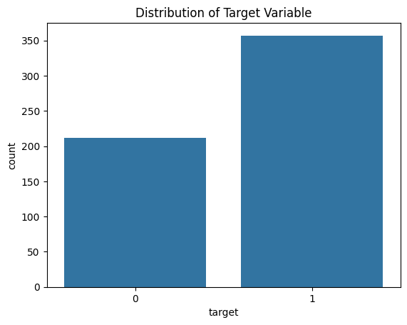

yozzum