[머신러닝] 모델평가

모델 평가

회귀모델 평가

실제 값과 에러치를 계산
회귀모델 : 예측의 결과가연속된 값으로 나타나는 것

분류모델 평가

평가항목
정확도(accuracy), 오차행렬(confusion matrix), 정밀도(precision), 재현율(recall),F1 score, ROC AUC
분류모델 : 고양이인지 강아지인지 구분, 아이리스 품종 맞추기

이진 분류 모델 평가

1인지 0인지 분류

이진 모델 예측 결과
TP True Positive : 실제 positive를 positive로 맞춘 경우
FN False Negative : 실제 positive를 negative라고 틀리게 예측한 경우 ((type 2 error)
TN True Negative : 실제 negative를 negative라고 맞춘 경우
FP False Positive : 실제 negative를 positive라고 틀리게 예측한 경우 (type 1 error)

이진 분류에서
actual values : true or false
predicted values : positive or negative

모델을 평가하는 수치들을 알아보자

Accuracy

accuracy = TP + TN/(TP+TN+FP+FN)
전체 데이터 중 맞게 예측한 것의 비율

Precision

precision = TP/(TP+EP)
양성이라고 예측한 것 중에서 실제 양성 비율
내가 실제 1이라고 말한 것 중에서 실제 1의 비율
정밀도를 높이기 위해서는 아주 확실할 때만 1로,,

FALL-OUT (FPR FALSE POSITION RATIO)

fallout = FP/(FP+TN)
실제 양성이 아닌데, 양성이라고 잘못 예측한 경우
실제 0중에서 1이라고 잘못 예측

Recall(TPR TRUE POSITIVE RATIO)

recall = TP/(TP+FN)
참인 데이터들 중에서 참이라고 예측한 것
놓쳐서는 안될 1을 신경써야할 때 봐야함

분류모델은 그 결과를 속할 비율(확률)을 반환한다.
지금까지는 그 비율에서 threshold를 0.5라고 보고, 결과를 0 또는 1로 반환했다.(이진분류에서)
iris의 경우 가장 높은 확률값이 있는 클래스를 해당값이라고 했다.

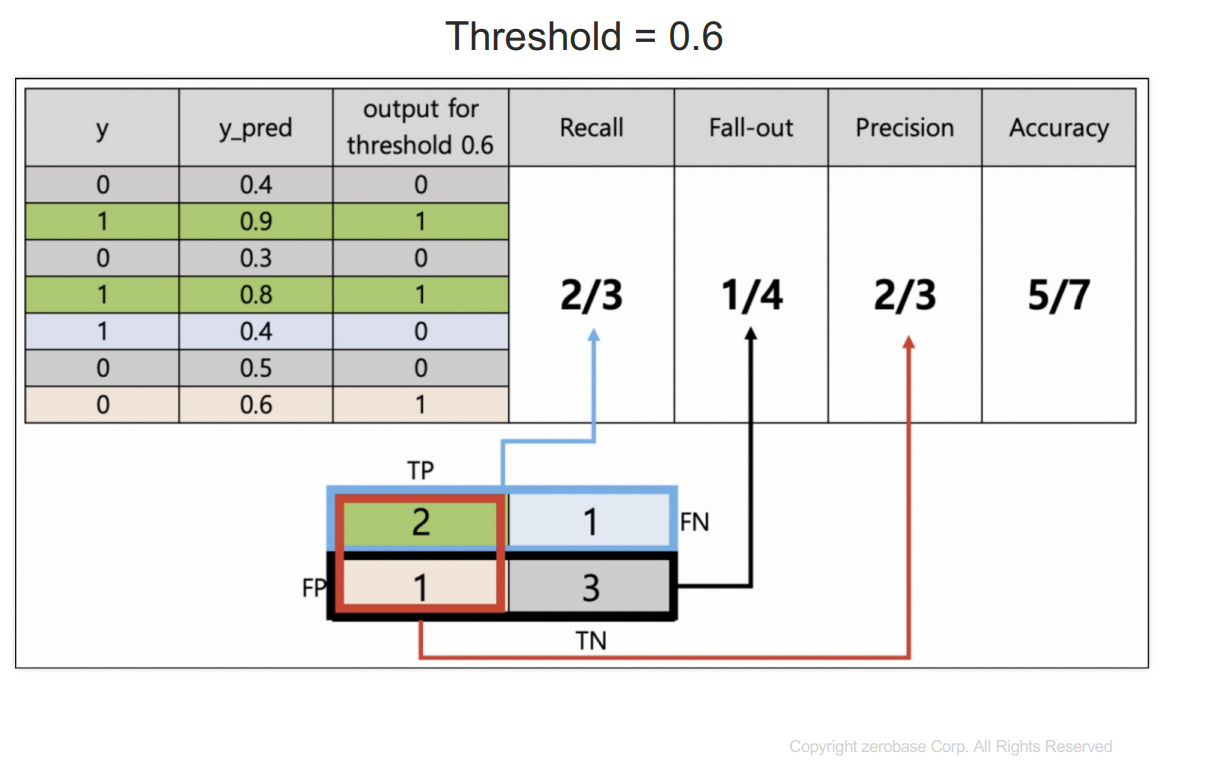
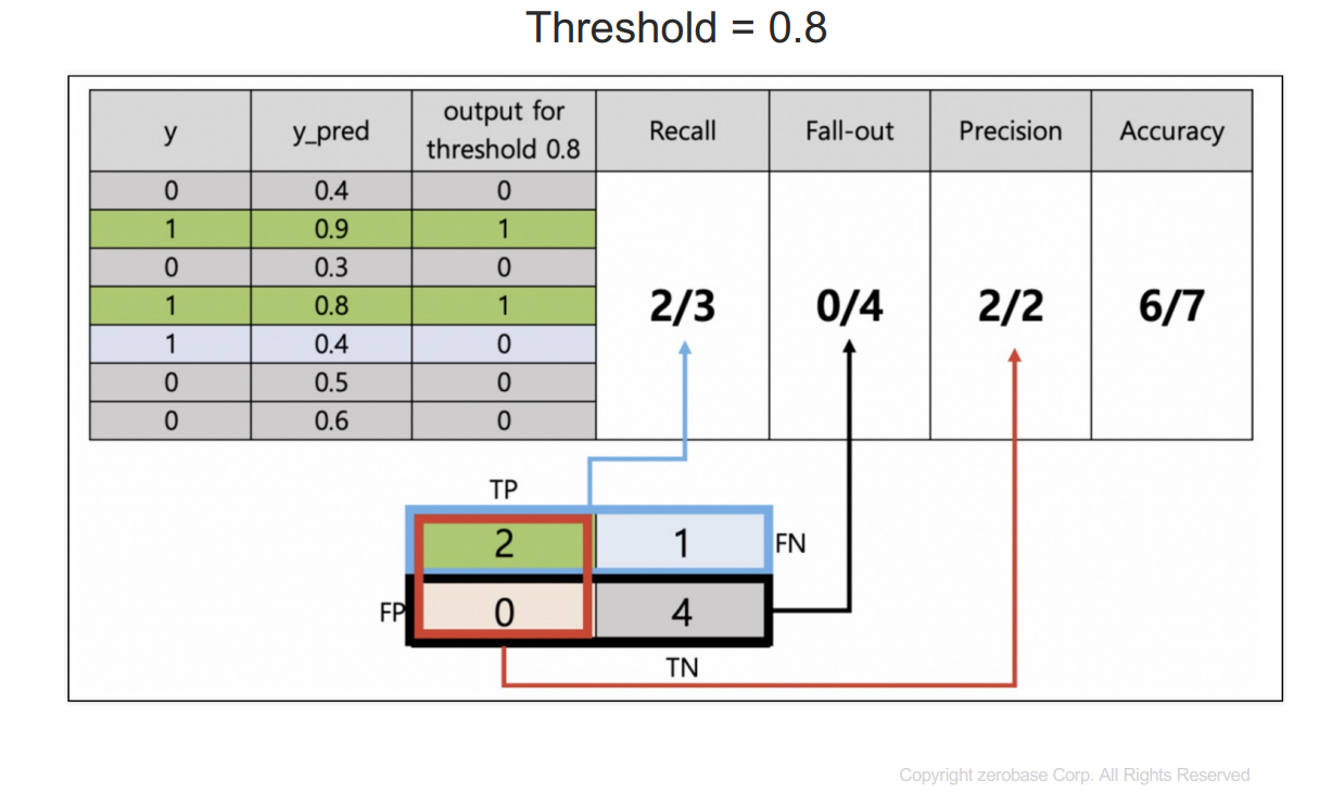
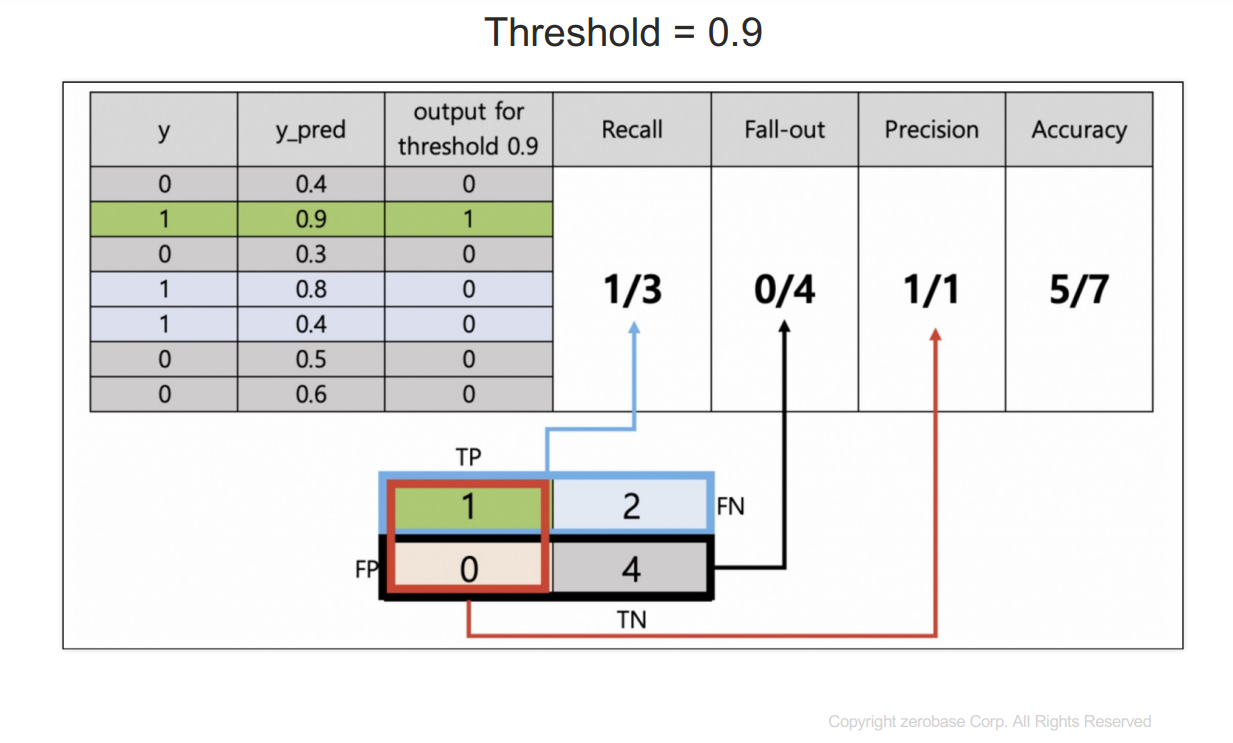
threshold를 변경해가면서 모델 평가 지표들을 관찰해보자.
y : 참값
y_pred : 1이 될 확률을 예측한 것
threshold보다 크거나 같으면 1이라고 예측한다.
recall : 실제 1인 데이터 중에서 1이라고 예측한 것
fall-out : 실제 0인데 1이라고 예측한 것
precision : 1이라고 예측한 것 중에 실제 1인 것
accuracy : 전체 데이터의 정확성

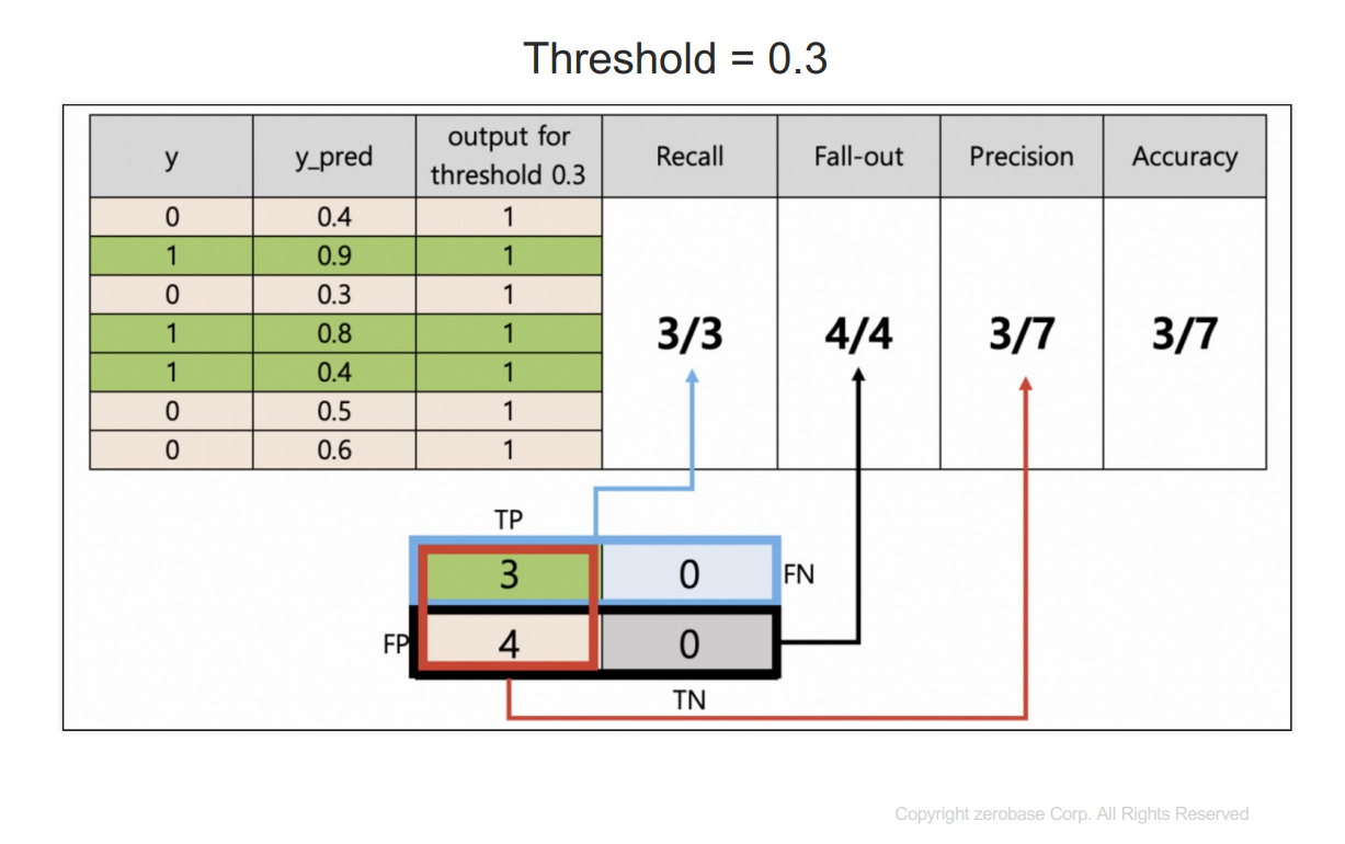
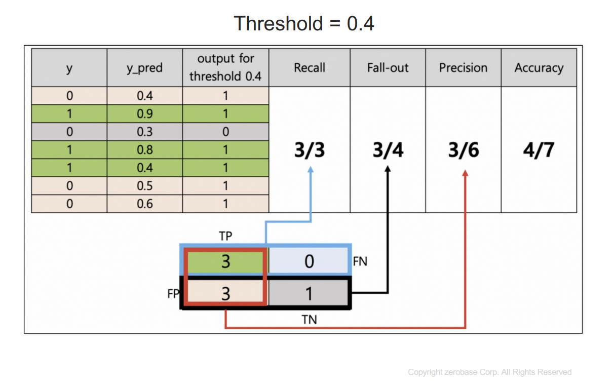
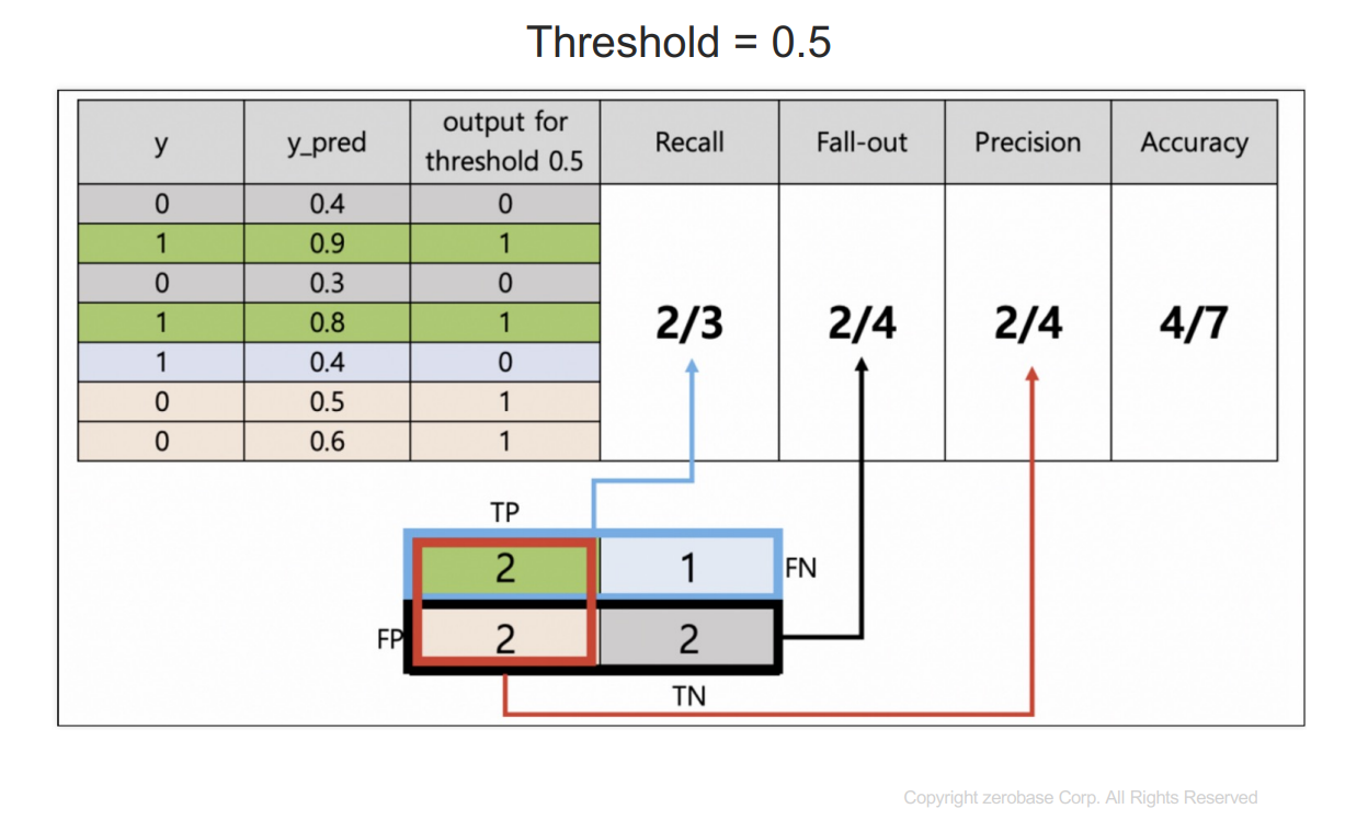
이를 정리하면
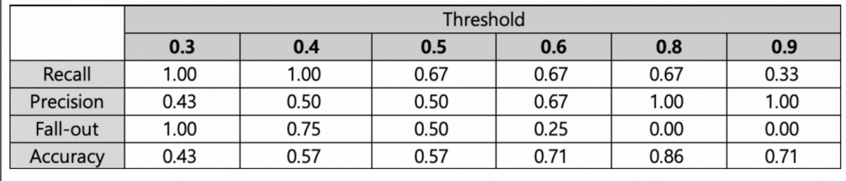recall은 참인 데이터 중 참이라고 예측한 데이터 비율
precision은 참이라고 예측한 것 중에서 실제 참인 데이터 비율을 말한다.
실제 양성인 데이터를 음성이라고 판단하면 안되는 경우(ex. 암환자 판별) recall이 중요하고
이 경우 threshold를 0.3 or 0.4로 선정해야 한다.
실제 음성인 데이터를 양성이라고 판단하면 안되는 경우(ex. 스팸메일 분류) precision이 중요하고 이 경우 threshold는 0.8 or 0.9가 적합하다.
그러나 recall과 precision은 서로 영향을 주기 때문에 한 쪽을 극단적으로 높게 설정하면 안된다.

F1-Score

recall, precision을 결합한 지표
recall, precision이 어느 한쪽으로 치우치지 않고 둘다 높은 값을 가지면 높은 값을 가짐
$F_β = (1+β^2)(precision * recall) / (β^2precision+recall)$
F-Score에서 beta를 1로 두면 F1-score
$F_1 = 2*precision*recall /(precision+recall)$

위 데이터에서 F1-Score를 계산하면
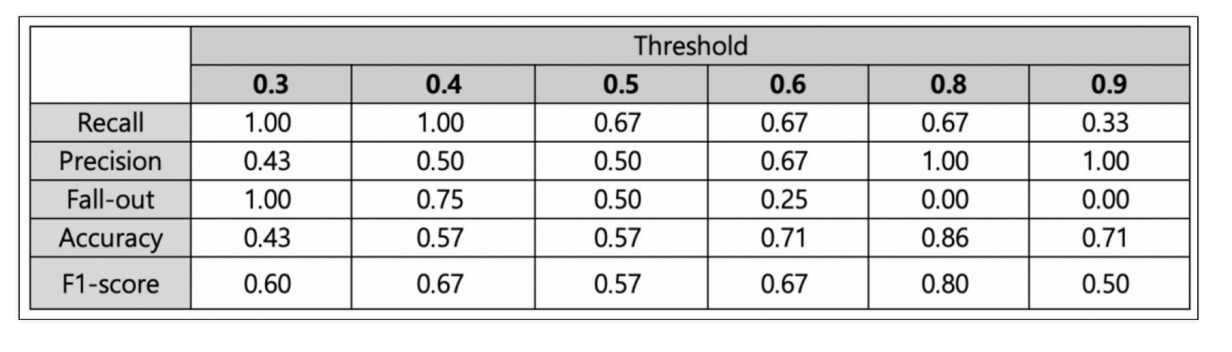recall과 precision을 모두 고려하면(F1-score가 가장 큰 값) threshold는 0.8이 적합하다.

ROC

ROC 곡선

• FPR(False Positive Rate, fall-out)이 변할 때,
  TPR(True Positive Rate, recall, sensitivity)의 변화를 그린 그림
• FPR을 x축, TPR을 y축으로 놓고 그림
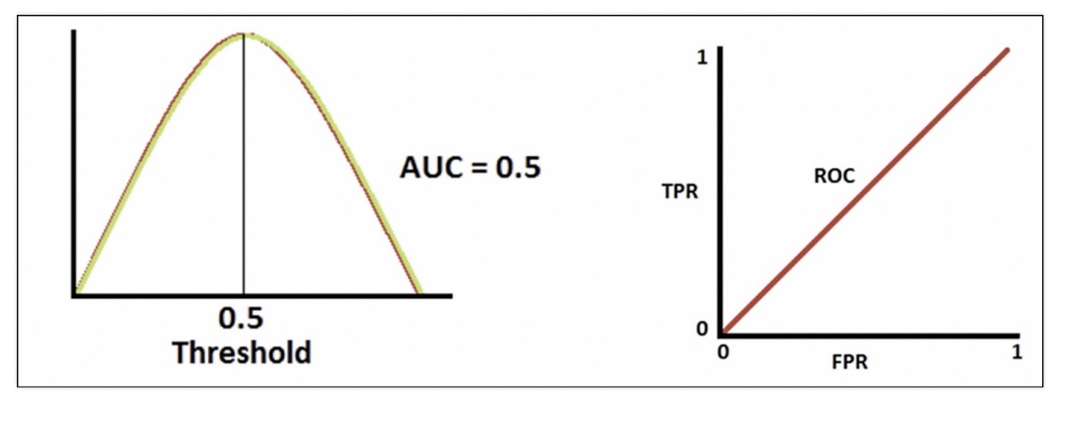
• 직선에 가까울 수록 머신러닝의 모델 성능이 떨어지는 것으로 판단
• 기울기 1에 가까운 직선형태로 나온다면
  아무 의미 없는 random하게 맞추기 해도 나옴
  직선이 위로 올라갈수록 좋은 모델이고, 위로 올라가서 꺾이면 더 좋다.
• AUC는 ROC 곡선 아래 면적

완벽하게 분류했다면
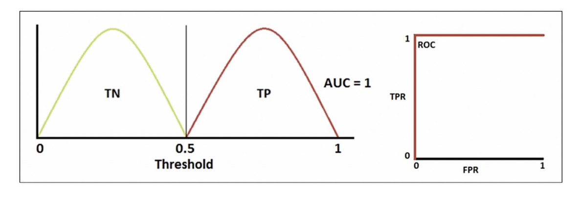TN, TP 경계선이 완전히 명확하고, ROC곡선에서 100% 다 맞추었다.

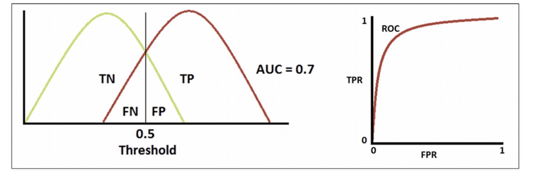
적당히 잘 분류했다면
분류 성능이 나쁘다면

ROC 곡선
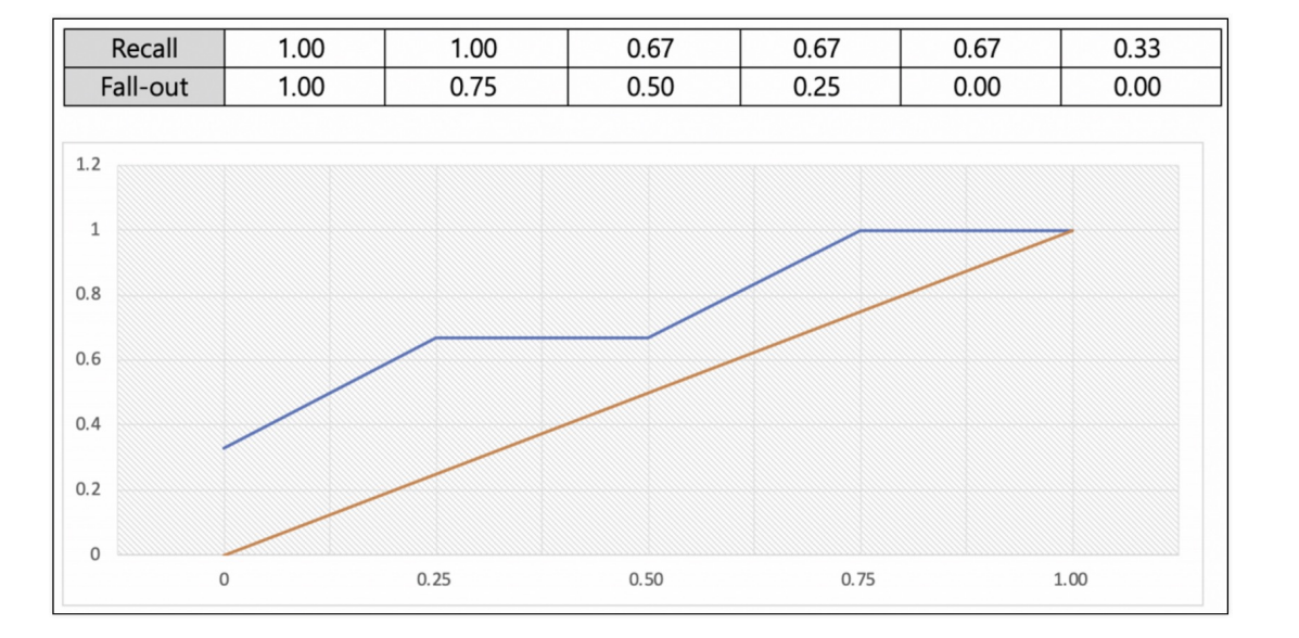AUC는 ROC 곡선(파란선) 아래 면적
AUC는 1에 가까울수록 좋은 수치
기울기가 1인 직선 아래 면적은 0.5이므로 AUC는 0.5보다 커야함

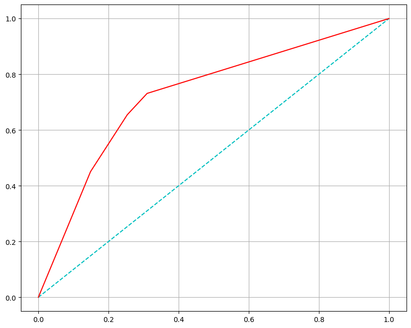
ROC 커브 그려보기

와인 데이터를 불러와서 ROC 커브를 그려보자

#와인데이터 불러오기
import pandas as pd

red_url = 'https://raw.githubusercontent.com/PinkWink/ML_tutorial/master/dataset/winequality-red.csv'
white_url = 'https://raw.githubusercontent.com/PinkWink/ML_tutorial/master/dataset/winequality-white.csv'

red_wine = pd.read_csv(red_url, sep=';')
white_wine = pd.read_csv(white_url, sep=';')

red_wine['color'] = 1
white_wine['color'] = 0

wine = pd.concat([red_wine, white_wine])
wine['taste'] = [1. if grade > 5 else 0. for grade in wine['quality']]

X = wine.drop(['taste', 'quality'], axis=1)
y = wine['taste']

#결정나무
from sklearn.model_selection import train_test_split
from sklearn.tree import DecisionTreeClassifier
from sklearn.metrics import accuracy_score

X_train, X_test, y_train, y_test = train_test_split(X, y, test_size=0.2, random_state=13)

wine_tree = DecisionTreeClassifier(max_depth=2, random_state=13)
wine_tree.fit(X_train, y_train)

y_pred_tr = wine_tree.predict(X_train)
y_pred_test = wine_tree.predict(X_test)

print('Train Acc : ', accuracy_score(y_train, y_pred_tr))
print('test Acc : ', accuracy_score(y_test, y_pred_test))

# 각 수치 구해보기
from sklearn.metrics import accuracy_score, precision_score
from sklearn.metrics import recall_score, f1_score
from sklearn.metrics import roc_auc_score, roc_curve

print('Accuracy : ', accuracy_score(y_test, y_pred_test))
print('Recall : ', recall_score(y_test, y_pred_test))
print('Precision : ', precision_score(y_test, y_pred_test))
print('AUC Score : ', roc_auc_score(y_test, y_pred_test))
print('F1 Score : ', f1_score(y_test, y_pred_test))

#ROC 커브 그리기
import matplotlib.pyplot as plt
%matplotlib inline

#모델 평가 수치 개념설명에서 나온 표에 y_pred, 1일 확률만 가져오기 위해서
pred_proba = wine_tree.predict_proba(X_test)[:, 1]
fpr, tpr, thresholds = roc_curve(y_test, pred_proba)

plt.figure(figsize=(10,8))
plt.plot([0,1], [0,1], 'c',ls='dashed') # (0,0), (1,1) 좌표를 지나는 직선
plt.plot(fpr, tpr, 'r')
plt.grid()
plt.show()