Control Hazard in Detail, how can minimize?

1. Simply Stalling
- Wait until previous instruction's WB ends, and insert nop.
2. Stalling makes more execution time.
When a branch instruction is encountered in a pipeline, such as a conditional branch like beq or bne, the processor faces a control hazard. To minimize this, the pipeline typically stalls, inserting no-operation (nop) instructions until the branch condition is resolved. However, stalling prolongs execution time because it delays subsequent instructions that could proceed independently.
Sol1. Minimize control-related instructions

1. Just guessing nextPC = PC + 4
2. Predicate Combining
- Get rid of unnecessary control flow instructions.
3. Predicated Execution
- Convert control dependences into data dependences.
With Predicate Combining, we aim to combine multiple predicates to minimize branching. With Predicated Execution, we convert control dependences into data dependences using conditional operations.
2. Predicate Combining
- Before
sub $t8, $t0, $t1       # $t8 = a - b
bgtz $t8, true_block1   # if a > b, go to true_block1
# false_block1
sub $t9, $t2, $t3       # $t9 = d - e
bgtz $t9, true_block2   # if d > e, go to true_block2
# false_block2
add $t7, $t5, $t6       # f = g + h
j end                   # jump to end
true_block2:
sub $t7, $t5, $t6       # f = g - h
j end                   # jump to end
true_block1:
add $t4, $t2, $t3       # c = d + e
j end                   # jump to end
end:
Branch misprediction penalties arise from the bgtz instructions in the control flow, which modern processors handle using branch predictors. Incorrect predictions result in pipeline flushes, discarding partially executed instructions and reloading with the correct path's instructions, leading to pipeline stalls and performance degradation. The original code contains two branches (bgtz for true\_block1 and true\_block2), each potentially mispredicted, doubling the chance of pipeline stalls. This increases pipeline flushes and control flow complexity, heightening the prediction difficulty and likelihood of mispredictions. Predicate combining simplifies control flow by merging multiple conditions and reducing the number of branches, thereby optimizing performance.
- After
sub $t8, $t0, $t1       # $t8 = a - b
slt $t9, $t0, $t1       # $t9 = 1 if a < b, 0 otherwise

sub $t10, $t2, $t3      # $t10 = d - e
slt $t11, $t2, $t3      # $t11 = 1 if d < e, 0 otherwise

# Calculate all possible outcomes
add $t4, $t2, $t3       # temp_c = d + e
sub $t7, $t5, $t6       # temp_f1 = g - h
add $t12, $t5, $t6      # temp_f2 = g + h

# Use the predicates to select the correct outcomes
movz $t7, $t12, $t11    # if $t11 == 0 (d >= e), $t7 = temp_f2
movn $t7, $t7, $t9      # if $t9 != 0 (a > b), $t7 = temp_f1

movn $t4, $t4, $t9      # if $t9 != 0 (a > b), $t4 = temp_c

end:
3. Predicated Execution
Using bgtz with a temporary register like $t9 to minimize control dependency is a strategy aimed at reducing the impact of branch mispredictions in the pipeline. By employing a conditionally executed instruction (bgtz) rather than a branch, the processor can potentially avoid the penalties associated with branch prediction failures. This approach allows the processor to continue executing subsequent instructions without stalling while waiting for the branch outcome. However, it's important to note that this technique introduces dependencies on the evaluation of the condition ($t9 > 0), which must be accurately predicted to avoid performance degradation. Therefore, while it can improve pipeline efficiency by reducing stalls due to mispredictions, careful consideration is needed to balance the benefits with the potential risks of relying on accurate condition evaluation in hardware execution.
- Before
# Assuming registers $t0 = a, $t1 = b, $t2 = d, $t3 = e, $t4 = c, $t5 = g, $t6 = h, $t7 = f

# Original MIPS Code
sub $t8, $t0, $t1       # $t8 = a - b
bgtz $t8, true_block    # if a > b, go to true_block
# false_block
add $t7, $t5, $t6       # f = g + h
j end                   # jump to end
true_block:
add $t4, $t2, $t3       # c = d + e
end:- After
# Predicated Execution
sub $t8, $t0, $t1       # $t8 = a - b
slt $t9, $t8, $zero     # $t9 = (a <= b) ? 1 : 0
add $t4, $t2, $t3       # c = d + e
mul $t7, $t9, $t5       # t7 = (a <= b) ? g : 0
mul $t10, $t9, $t6      # t10 = (a <= b) ? h : 0
add $t7, $t7, $t10      # f = g + h if a <= b
Sol2. Delayed Branching

1. Inserting nop.
2. Reordering, filling branch delay slot.
Both methods aim to reduce pipeline stalls caused by branch instructions. Inserting NOPs is straightforward but adds idle cycles in the pipeline. Reordering instructions to fill the delay slot can potentially improve performance by keeping the pipeline busy with useful instructions. The choice between these methods often depends on the specific pipeline design and the characteristics of the branch instructions.
Misprediction Penalty


Misprediction penalty refers to the additional delay incurred by a CPU when a branch prediction fails. When a branch instruction (e.g., conditional jump, branch command) is encountered, the CPU predicts the next instruction's address to optimize performance. If this prediction turns out to be incorrect, the CPU must discard the current execution path and redirect to the correct instruction, resulting in a penalty of typically 3 cycles, known as "3 bubbles." During this time, the CPU prepares to jump to the correct address and fetches the correct instruction, effectively introducing idle cycles into the execution pipeline. Efficient branch prediction algorithms are crucial in minimizing misprediction penalties and optimizing CPU performance.
Sol3. Static Branch Prediction
Branch prediction strategies play a crucial role in optimizing the performance of modern processors by predicting the outcome of conditional branches before their actual execution. Here are some key strategies:
- Always taken
- This strategy predicts that all branches will be taken, meaning control flow will always follow the branch instructions. This approach is beneficial when branches are predominantly taken, reducing the risk of mispredictions but potentially causing inefficiencies when branches are not taken.
- Always not taken
- In contrast, this strategy assumes that all branches will not be taken, meaning control flow proceeds to the next sequential instruction after a branch instruction unless explicitly redirected by the branch condition. This strategy is effective when branches are rarely taken, minimizing misprediction penalties but possibly failing to exploit opportunities for optimization in branches that are frequently taken.
- BTFN (Backward Taken, Forward Not Taken)
- BTFN predicts that backward branches (branches to lower memory addresses) are taken and forward branches (branches to higher memory addresses) are not taken. This strategy leverages typical program control flow patterns where loops tend to have backward branches and conditional checks tend to have forward branches.
- Compiler-based and program-based
- Compiler-based strategies use static analysis performed by the compiler to predict branch outcomes based on heuristics and profiling data gathered during compilation. Program-based strategies rely on dynamic execution characteristics observed at runtime to adaptively predict branch outcomes.
Each strategy has trade-offs in terms of prediction accuracy and performance impact. Effective branch prediction improves processor throughput by minimizing stalls due to branch delays and reducing the penalties associated with mispredicted branches, thereby enhancing overall system efficiency.
- Implementation
# Determine if the instruction is a branch
if instruction.is_branch():
    # Apply static branch prediction based on prediction_mode
    if prediction_mode == "always_taken":
        taken = True
    elif prediction_mode == "always_not_taken":
        taken = False
    elif prediction_mode == "btfnt":
    # Backward Taken, Forward Not Taken
        if shred.pc > shred.if_id_latch.pc:  # Forward branch
            taken = False
        else:  # Backward branch
            taken = True
    else:
    # Default behavior, could be compiler-based or program-based prediction
    # Not explicitly implemented here
        taken = True  # Assume always taken as default

    # Check if prediction matches actual outcome
    if taken == (instruction.get_target_address() != shred.pc + 1):
        penalty = 3  # Misprediction penalty
    else:
        penalty = 0
Sol4. Dynamic Branch Prediction
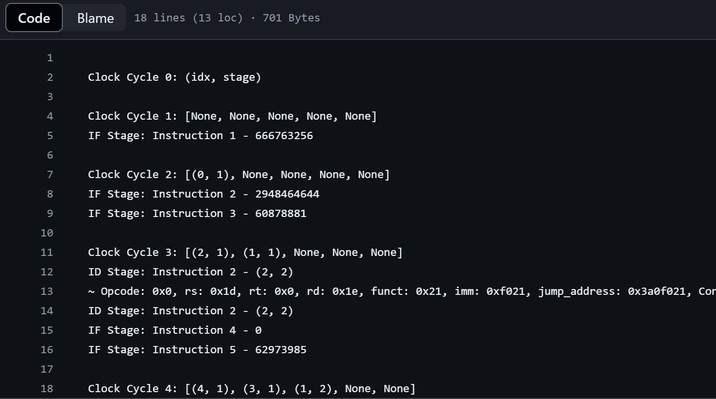
My code simulates a simple pipelined processor with a focus on branch prediction. It includes the Instruction class to model instructions and their attributes, such as opcode, destination register, source registers, program counter, and branch prediction details. The BranchTargetBuffer (BTB) class manages branch target entries and updates, while the LastTimePredictor (LTP) class handles branch prediction states. The pipeline stages (IF, ID, EX, MEM, WB) are implemented in separate functions, each processing instructions and updating the pipeline state. The Shred class initializes the pipeline with instructions and manages pipeline latches. The simulate\_pipeline function runs the simulation cycle-by-cycle, and the test\_pipeline function tests the pipeline, printing the final states of BTB and LTP.
In this code, a 2-bit counter is used within the Last Time Predictor (LTP) to improve branch prediction accuracy by tracking the state of branch instructions. The counter has four states: 0 (Strongly Not Taken), 1 (Weakly Not Taken), 2 (Weakly Taken), and 3 (Strongly Taken). When a branch is encountered, the LTP checks the counter state to predict the outcome. If the state is 2 or 3, the branch is predicted as taken; if the state is 0 or 1, it is predicted as not taken. After the branch outcome is known, the counter is updated: it increments if the branch was taken and decrements if it was not, ensuring that the predictor gradually adjusts to the actual behavior of branches.
- in Instruction class
self.target_address = 0  # Target address for branch instructions
self.branch_prediction = None  # Predicted outcome of the branch
self.branch_taken = None  # Actual outcome of the branch
self.predicted_target_address = None  # Predicted target address for branch instructions
self.predictor_state = 0  # Initial predictor state (Strongly not taken)
self.btb_valid = False  # Valid bit for BTB
self.btb_tag = None  # Tag to identify branch in BTB
self.ltp_history = 0  # History bits for LTP
These attributes are added to the Instruction class to facilitate branch prediction and tracking within the pipeline. self.branch\_prediction stores the predicted outcome of a branch instruction, while self.branch\_taken records the actual outcome after execution. self.predicted\_target\_address holds the predicted target address for branch instructions. self.predictor\_state represents the current state of the 2-bit counter used in the Last Time Predictor (LTP). self.btb\_valid indicates if the Branch Target Buffer (BTB) entry is valid, and self.btb\_tag helps identify branches in the BTB. Finally, self.ltp\_history keeps track of the branch history bits for the LTP. These attributes collectively enable accurate branch prediction and update mechanisms within the pipeline stages.
- in BranchTargetBuffer class
class BranchTargetBuffer:
    def __init__(self, size):
        self.size = size
        self.entries = [None] * size  # Initialize BTB entries with None

    def get_entry(self, pc):
        index = pc % self.size
        return self.entries[index]

    def update_entry(self, pc, target_address):
        index = pc % self.size
        self.entries[index] = (pc, target_address)  # Store both PC and target address

    def update_tag(self, pc, tag):
        index = pc % self.size
        if self.entries[index] is not None:
            self.entries[index] = (tag, self.entries[index][1])  # Update tag only
This BranchTargetBuffer class provides a mechanism to store and manage target addresses for branch instructions in a processor. It initializes with a specified size and uses an array (entries) to store tuples of (PC, target address). Methods include get\_entry to retrieve entries based on PC, update\_entry to store PC and target address pairs, and update\_tag to update tags in existing entries based on PC. This class supports efficient branch prediction by storing and retrieving target addresses quickly using modulo indexing.
- in LastTimePredictor class
class LastTimePredictor:
    def __init__(self):
        self.predictor_table = {}

    def predict_branch(self, instruction):
        if instruction.pc in self.predictor_table:
            state = self.predictor_table[instruction.pc].predictor_state
            if state >= 2:
                return True
            else:
                return False
        else:
            return False  # Default not taken for new branches

    def update_branch_prediction(self, instruction):
        if instruction.pc not in self.predictor_table:
            self.predictor_table[instruction.pc] = instruction
        else:
            state = self.predictor_table[instruction.pc].predictor_state
            if instruction.branch_taken:
                state = min(state + 1, 3)  # Strongly taken (3), Weakly taken (2)
            else:
                state = max(state - 1, 0)  # Weakly not taken (1), Strongly not taken (0)
            self.predictor_table[instruction.pc].predictor_state = state
This LastTimePredictor class implements a 2-bit counter-based branch prediction mechanism. It maintains a predictor\_table to store the prediction states for different program counters (PCs). The predict\_branch method predicts the outcome of a branch instruction based on the stored state in predictor\_table. If the PC exists in predictor\_table and the state is 2 or higher, it predicts the branch as taken; otherwise, it predicts it as not taken. The update\_branch\_prediction method updates the predictor state based on the actual outcome (branch\_taken) of the branch instruction. It adjusts the state upwards for taken branches and downwards for not taken branches, ensuring the predictor adapts to changing branch behavior over time. This class effectively enhances branch prediction accuracy by dynamically adjusting predictions using historical behavior stored in the 2-bit counters.
