시계열 모형 종류

• AR(p) - 자기 회귀 모형 ,AR(1)에 적용하기 위해선 −1<ϕ1<1조건이 필요하다
• MA(q) - 이동평균 모형
• ARMA(p,q)
• ARIMA(p,d,q) - 자기회귀누적이동평균 모형 : 차수의 개수(d)는 거의 2를 넘지 않는다.
• SARIMA(Seasonal ARIMA) - 계절 자기회귀이동평균 모형

▪ AR – 자기회기 모형

• AR(Autoregressive) 모델은 자기회귀(Autoregressive) 모델로 자기상관성을 시계열 모델로
구성한 것이다.
• 예측하고 싶은 특정 변수의 과거 자신의 데이터와 선형 결합을 통해 특정 시점 이후 미래값을
예측하는 모델이다.
• 이름 그대로 이전 자신의 데이터가 이후 자신의 미래 관측값에 영향을 끼친다는 것을 기반으로
나온 모델이다.
• AR(1)에 적용하기 위해선 −1<ϕ1<1조건이 필요하다.

# ArmaProcess로 모형 생성하고 nobs 만큼 샘플 생성
from statsmodels.tsa.arima_process import ArmaProcess

def gen_arma_samples (ar,ma,nobs): 
    arma_model = ArmaProcess(ar=ar, ma=ma) # 모형 정의
    arma_samples = arma_model.generate_sample(nobs) # 샘플 생성
    return arma_samples
# drift가 있는 모형은 ArmaProcess에서 처리가 안 되어서 수동으로 정의해줘야 함
def gen_random_walk_w_drift(nobs,drift): 
    init = np.random.normal(size=1, loc = 0) 
    e = np.random.normal(size=nobs, scale =1) 
    y = np.zeros(nobs) 
    y[0] = init
    for t in (1,nobs): 
        y[t] = drift + 1 * y[t-1] + e[t] 
        return y
        

## AR 모형
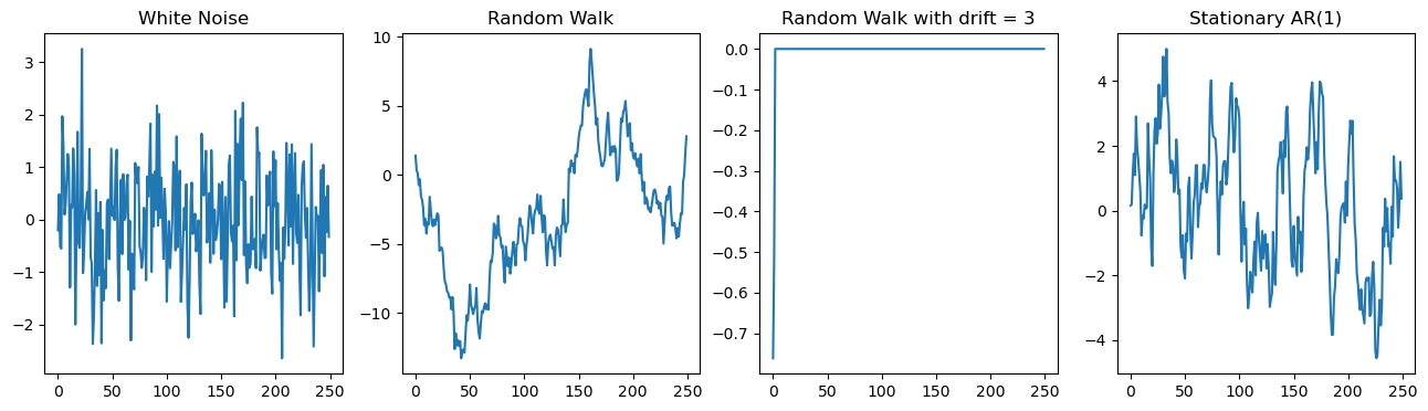
np.random.seed(12345)

white_noise= gen_arma_samples(ar = [1], ma = [1], nobs = 250) 
# y_t = epsilon_t

random_walk = gen_arma_samples(ar = [1,-1], ma = [1], nobs = 250) 
# (1 - L)y_t = epsilon_t

random_walk_w_drift = gen_random_walk_w_drift(250, 2) 
# y_t = 2 + y_{t-1} + epsilon_t

stationary_ar_1 = gen_arma_samples(ar = [1,-0.9], ma = [1],nobs=250) 
# (1 - 0.9L) y_t = epsilon_t

import matplotlib.pyplot as plt

fig,ax = plt.subplots(1,4)
ax[0].plot(white_noise)
ax[0].set_title("White Noise")

ax[1].plot(random_walk)
ax[1].set_title("Random Walk")

ax[2].plot(random_walk_w_drift)
ax[2].set_title("Random Walk with drift = 3")

ax[3].plot(stationary_ar_1)
ax[3].set_title("Stationary AR(1)")

fig.set_size_inches(16,4)

MA 모형

## MA 모형
np.random.seed(12345)
ma_1 = gen_arma_samples(ar = [1], ma = [1,1], nobs = 250) # y_t = (1+L) epsilon_t
ma_2 = gen_arma_samples(ar = [1], ma = [1,0.5], nobs = 250) # y_t = (1+0.5L)epsilon_t
ma_3 = gen_arma_samples(ar = [1], ma = [1,-2], nobs = 250) # y_t = (1-2L) epsilon_t
fig,ax = plt.subplots(1,3, figsize = (12,4))
ax[0].plot(ma_1)
ax[0].set_title("MA(1) with theta_1 = 1")

ax[1].plot(ma_2)
ax[1].set_title("MA(1) with theta_1 = 0.5")

ax[2].plot(ma_3)
ax[2].set_title("MA(1) with theta_1 = -2")

plt.show()

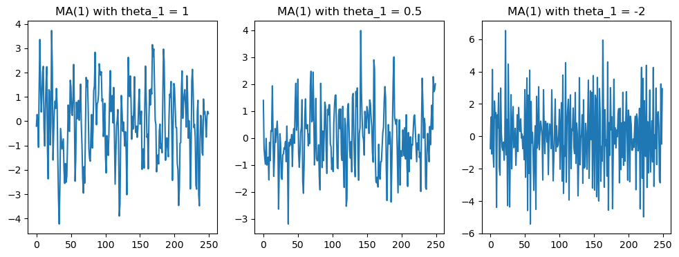
위 그림에서 볼 수 있듯이 θ1의 값에 따라 모형 형태가 약간 다르긴 하지만 특정한
트렌드도 없고 평균과 분산이 일정하기 때문에 정상성을 만족함을 확인하실 수 있다.