[CV] 12. Optical Flow

Week 12-2. Optical Flow

1. Motion Field and Optical Flow

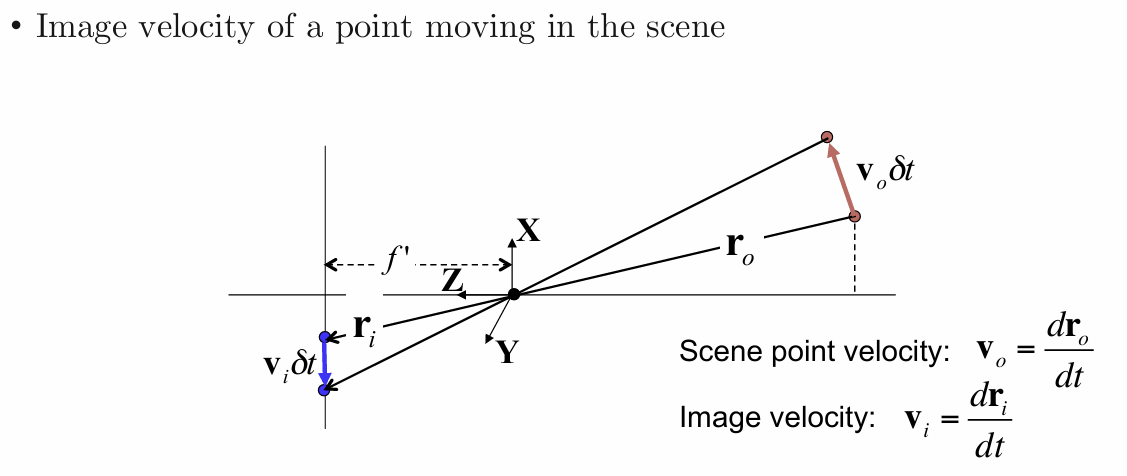
Motion Field
Image velocity of a point moving in the scene

Optical Flow
Motion of brightness pattern in the image
Ideally, Optical flow = Motion field
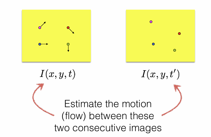
Problem Definition: Given two consecutive image frames, estimate the motion of each pixel
consecutive:

Optical Flow != Motion Field
제자리에서 돌아가면 motion field 있고 optical flow 없음
광원이 움직이면 motion field 없고 optical flow 있음
Barber pole illusion, Donguri wave illusion

2. Brightness Constancy Equation

Key Assumption
1. Brightness (Color) Constancy
implication: Allows for pixel to pixel comparison (not image features)
I(x(t),y(t),t) = C
2. Small Motion
pixels only move a little bit
implication: Linearization of the brightness constancy constraint
Look for nearby pixels(small motion) with the same color(brightness constancy)
$I(x+u\delta t,y + v\delta t,t + \delta t) = I(x,y,t)$

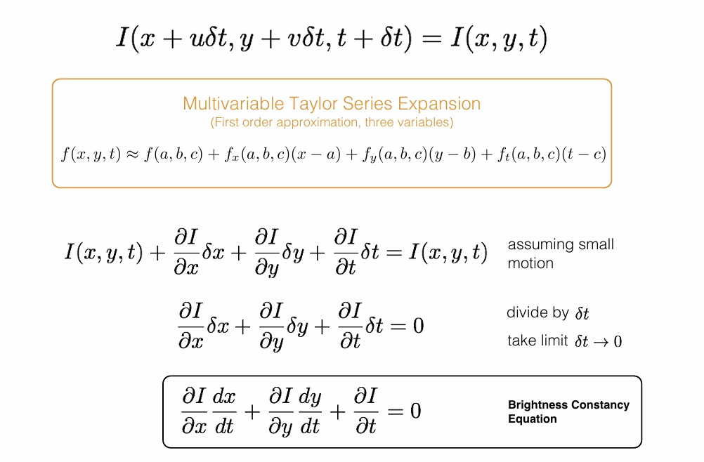
Brightness Constancy Equation
Insight: If the time step is really small, we can linearize the intensity function
크게 보면 곡선이어도 짧은 부분은 직선과 같다

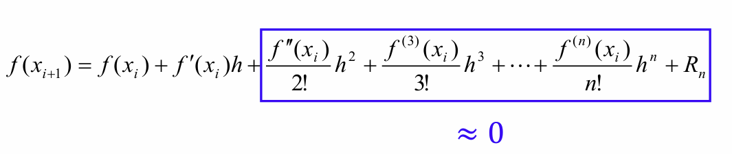
• Multivariable Taylor Series Expansion
  assuming small moiton
  cancel terms
  brightness constancy equation

shorthand notation $I_x u + I_y v + I_t = 0$
vector form $\nabla I^Tv + I_t = 0$

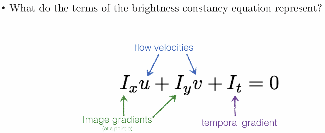
• How do you compute?
  u, v 직선 위에 있어 unique하게 결정 안 됨
  solution lies on a straight line

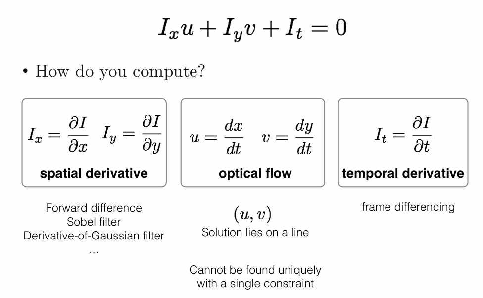
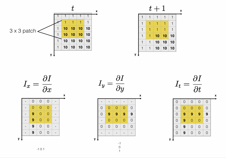
• Example
  t+1 - t = $I_t = \frac{\delta I}{\delta t}$ (forward difference)

3. Constant Flow (a.k.a. Lukas-Kanade Optical Flow)

Assumptions:
• Flow is locally smooth
• Neighboring pixels have same displacement
Using a 5×5 image patch, gives us 25 equations

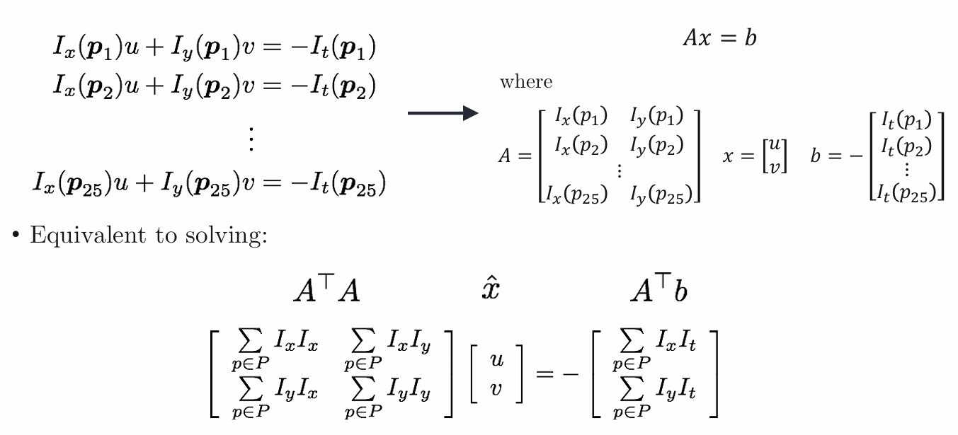
• Lucas-Kanade Optical Flow: $x = (A^TA)^{-1}A^Tb$

• Solvable:
  $A^TA$ invertible,
  not too small- $\lambda_1, \lambda_2$ not too small,
  well conditioned- $\lambda_1/ \lambda_2$ not too large

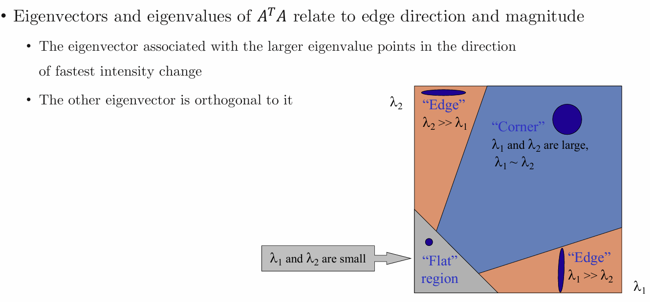
• Eigenvecotrs and eigenvalues of $A^TA$ relate to edge direction and magnitude

• Low-texture region (bad)
  : Gradients have small magnitude, small $\lambda_1,\lambda_2$

• Edges (so so)- Aperture problem
  gradients are very large or very small, Large $\lambda_1$, small $\lambda_2$

• high-texture region (good)
  : Gradients are different, large magnitude, Large $\lambda_1$, large $\lambda_2$

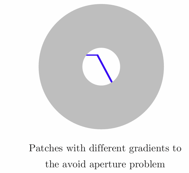
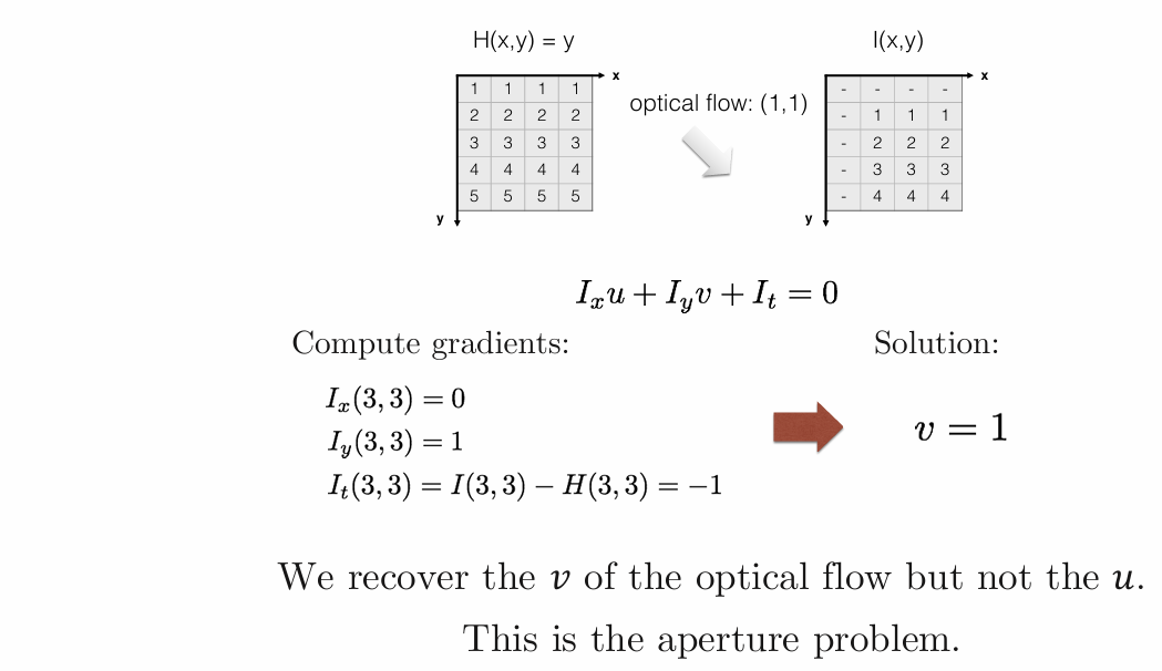
Aperture problem
v 구함, u 구해야함- 다음내용
-_ actual motion >
small visible image patch, preceived motion /^

4. Coarse-to-Fine Flow Estimation

What if we have large motion?
• Taylor series approximation is not valid.
Solution: Reduce the resolution!
u = 1.25, 2.5, 5, 10 pixels
Gaussian pyramid, run iterative L-K -> warp & upsample

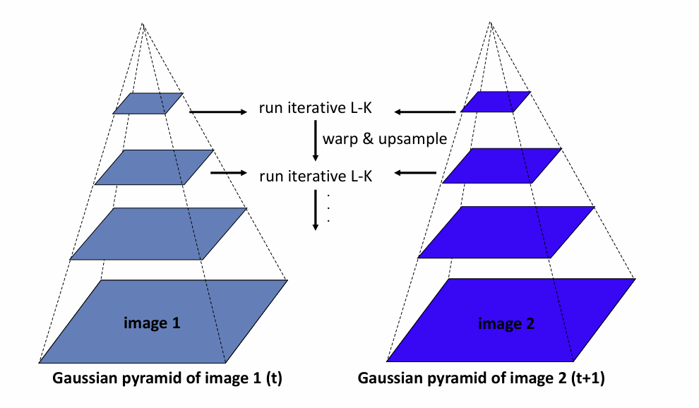
• Lukas-Kanade with pyrammids
  good

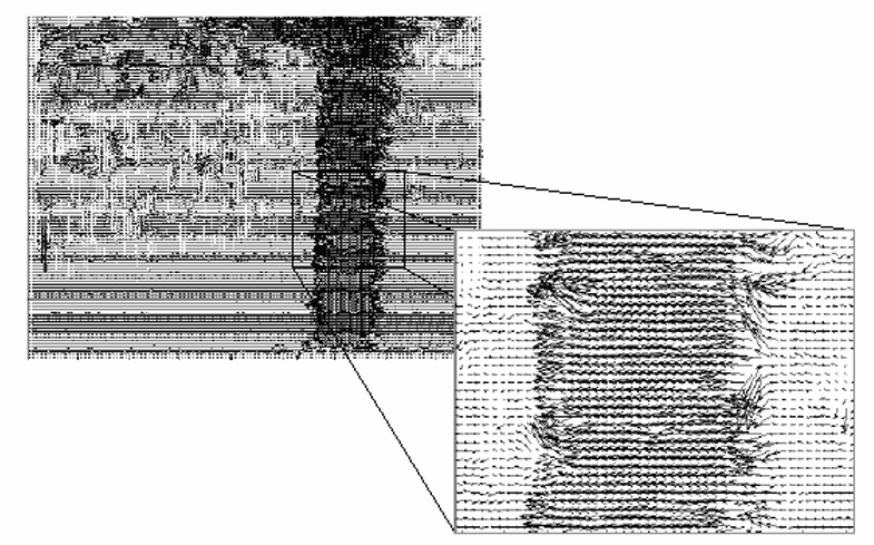
5. Applications of Optical Flow

Optical Mouse, Traffic Monitoring, Slow Motion Effect(Video Retiming), Video Stabilization