BG-NBD (기대 횟수 예측)

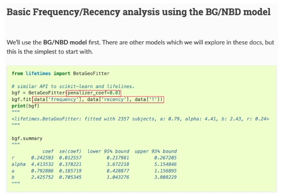
진행을 위해 필요한 최소한의 값 :

• frequency
• recency
• T (Time)

penalizer_coef는 모델 객체 초기화 시 사용하는 하이퍼 파라미터로, 복잡성을 제어하고 과적합을 컨트롤하는 데에 사용됨. 공식 문서에 따르면 0.001 - 0.1 사이의 값으로 설정하는 게 효과적이라고 함

Gamma-Gamma (기대 구매 금액 예측)

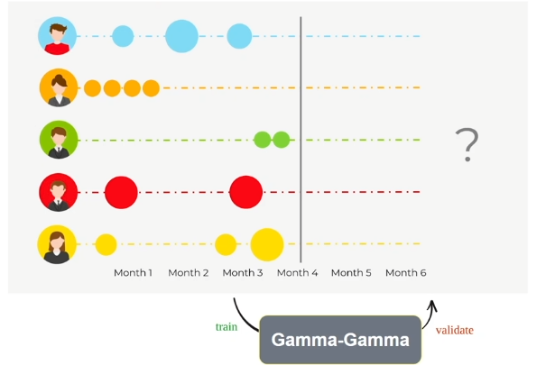
진행을 위해 필요한 최소한의 값 :

• frequency
• monetary

특히,
Frequency와 Monetary간 피어슨 상관관계가 0에 가까워야 함. 즉, 구매 빈도와 구매 금액 간의 상관관계가 거의 없어야 함.

여기서도 penalizer_coef는 모델 객체 초기화 시 사용하는 하이퍼 파라미터로, 복잡성을 제어하고 과적합을 컨트롤하는 데에 사용됨.

---

CLTV 예측

패키지 임포트

from lifetimes import BetaGeoFitter
from lifetimes import GammaGammaFitter

집계일 지정하기

df_cltv2 = df_cltv.copy()
target_date = df_cltv2['last_order_date'].max()
target_date

R, F, M, T 구하기

df_cltv2['frequency'] = df_cltv2['order_num_total']

# Recency : 고객별 첫 구매부터 마지막 구매까지의 시간
df_cltv2['recency'] = df_cltv2['last_order_date'] - df_cltv2['first_order_date']

# T(Time) : 고객별 첫 구매부터 집계일까지의 시간
df_cltv2['T'] = target_date - df_cltv2['first_order_date']

# 고객별 평균 금액
df_cltv2['Monetary'] = df_cltv2['customer_value_total'] / df_cltv2['order_num_total']

R과 T를 week 기준으로 변경하기

# recency와 T를 주차별로 재설정
df_cltv2['recency'] = df_cltv2['recency'].dt.days
df_cltv2['T'] = df_cltv2['T'].dt.days

df_cltv2['recency'] = df_cltv2['recency'] / 7
df_cltv2['T'] = df_cltv2['T'] / 7

# 모델 메서드 사용 기준이 주차별이므로

BG-NBD로 구매 횟수 예측

향후 1주 간의 구매 횟수 예측

# BG-NBD

bgf = BetaGeoFitter(penalizer_coef = 0.001)
bgf.fit(df_cltv2['frequency'], df_cltv2['recency'], df_cltv2['T'])

# conditional_expected_number_of_purchases_up_to_time:
# T 시점까지의 예상 구매 횟수 계산
bgf.conditional_expected_number_of_purchases_up_to_time(1, # 향후 1주 간의 예상 구매 횟수 출력
                                                        df_cltv2['frequency'],
                                                        df_cltv2['recency'],
                                                        df_cltv2['T']).sort_values(ascending=False).head(10)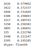                                                   

위 결과를 통해, 일주일 안에 0.57회를 구매해야 구매 횟수에서 1등인 것을 알 수 있음

향후 1달(=4주)간의 구매 횟수 예측

# 한 달 간의 예상 구매 횟수 출력
bgf.conditional_expected_number_of_purchases_up_to_time(4, # 향후 1달(=4주) 간의 예상 구매 횟수 출력
                                                        df_cltv2['frequency'],
                                                        df_cltv2['recency'],
                                                        df_cltv2['T']).sort_values(ascending=False).head(10)                                                   

향후 반 년(=6개월) 간의 구매 횟수 예측

# 반 년 간의 예상 구매 횟수 출력
bgf.conditional_expected_number_of_purchases_up_to_time(4 * 6, # 향후 반년 간의 예상 구매 횟수 출력
                                                        df_cltv2['frequency'],
                                                        df_cltv2['recency'],
                                                        df_cltv2['T']).sort_values(ascending=False).head(10)                                                   

Gamma-Gamma와 BG-NBD로 고객 생애 가치(CLTV) 예측

# Gamma-Gamma 모델 fitting
ggf = GammaGammaFitter(penalizer_coef=0.01)
ggf.fit(df_cltv2['frequency'], df_cltv2['Monetary'])

# 6개월의 고객 생애 가치 예측
df_cltv2['cltv_pred_6months'] = ggf.customer_lifetime_value(bgf,
                                                           df_cltv2['frequency'],
                                                           df_cltv2['recency'],
                                                           df_cltv2['T'],
                                                           df_cltv2['Monetary'],
                                                           time=6, # 6 months
                                                           freq='W', # T의 기준은 '주차'별이므로, week을 의미하는 W
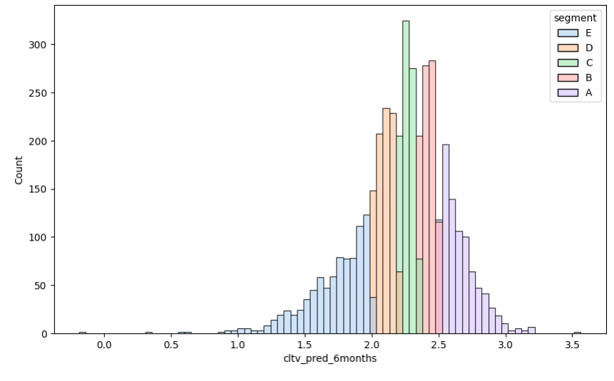
                                                           discount_rate=0.01)

CLTV로 등급 정하기

df_cltv2['segment'] = pd.qcut(df_cltv2['cltv_pred_6months'], 5, labels=['E', 'D', 'C', 'B', 'A'])
df_cltv2.head()

CLTV 등급 시각화

plt.figure(figsize=(10,6))
sns.histplot(x=np.log10(df_cltv2['cltv_pred_6months']),
            hue=df_cltv2['segment'],
            palette='pastel')
plt.show()