1 Pandas
1.1 판다스(Pandas)
- Python Data Analysis Library의 약어
- R의 data.frame을 벤치마킹하여 Python에서 사용할 수 있는 형태의 Dataframe을 제공해주는 라이브러리
- Python을 활용해 데이터 분석을 하기 위해서 사용하는 필수적인 패키지
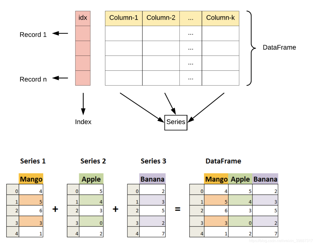
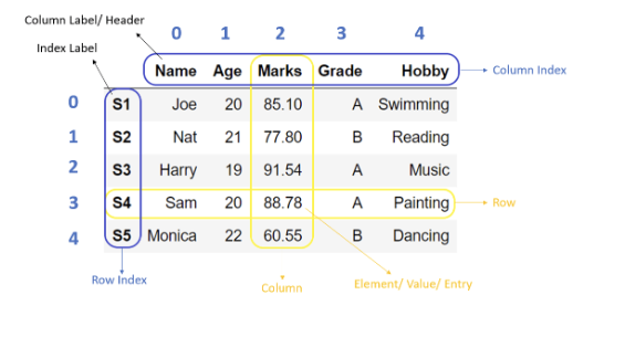
1.2 데이터프레임 구조 및 명칭
필요한 패키지 import 하기
	import numpy as np
	import pandas as pd
2 데이터프레임 다루기(기초)
2.1 데이터프레임 생성하기
- pandas.DataFrame()
- data : dict, list, set, ndarray, lterable 또는 DataFrame
- [index] : index명, 디폴트는 0, 1, 2..
- [columns] : 컬럼명, 디폴트는 0, 1, 2..
- [dtype] : 데이터 타입 지정
- [copy] : 입력으로부터 복사, True or False
직접 데이터프레임 작성하기
	my_df = pd.DataFrame(data=np.array([[1, 2, 3], [4, 5, 6]])
                         , index=range(1,3), columns=['A','B','C'])
    print(my_df)
결과
A B C
1 1 2 3
2 4 5 62D array를 데이터프레임으로 변환
    my_2darray = np.array([[1, 2, 3], [4, 5, 6]])
	print(pd.DataFrame(my_2darray))
결과
0 1 2
0 1 2 3
1 4 5 6dictionary를 데이터프레임으로 변환
	my_dict = {'a': ['1', '3'], 'b': ['1', '2'], 'c': ['2', '4']}
	print(pd.DataFrame(my_dict))
결과
a b c
0 1 1 2
1 3 2 4Series를 데이터프레임으로 변환
	my_series = pd.Series({'United Kingdom':'London', 'India':'New Delhi'
                       , 'United States':'Washington', 'Belgium':'Brussels'})
	print(pd.DataFrame(my_series))
결과
0
United Kingdom London
India New Delhi
United States Washington
Belgium Brussels
외부 파일로 부터 불러오기
	df = pd.read_csv('bank.csv', sep = ',')
	print(df.head(3)) # default=5
결과
age;"job";"marital";"education";"default";"balance";"housing";"loan";"contact";"day";"month";"duration";"campaign";"pdays";"previous";"poutcome";"y"
0 30;"unemployed";"married";"primary";"no";1787;...
1 33;"services";"married";"secondary";"no";4789;...
2 35;"management";"single";"tertiary";"no";1350;... 2.2 데이터프레임 살펴보기
메타데이터 확인하기
	my_df = pd.DataFrame(data=np.array([[1, 2, 3], [4, 5, 6]])
                     , index=range(1,3), columns=['A','B','C'])
	my_df.info()
결과
<class 'pandas.core.frame.DataFrame'>
RangeIndex: 2 entries, 1 to 2
Data columns (total 3 columns):
#Column Non-Null Count Dtype
--- ------ -------------- -----
0 A 2 non-null int32
1 B 2 non-null int32
2 C 2 non-null int32
dtypes: int32(3)
memory usage: 156.0 bytes출력 제한 걸기
	pd.options.display.max_rows = 20  # 최대 표시 행수
    pd.set_option('display.min_rows', 5) # 최소 표시 행수

    df = pd.read_csv('bank.csv', sep = ',').iloc[:,0:7]
    print(df)
결과
age job marital education default balance housing
0 58 management married tertiary no 2143 yes
1 44 technician single secondary no 29 yes
... ... ... ... ... ... ... ...
45209 57 blue-collar married secondary no 668 no
45210 37 entrepreneur married secondary no 2971 no
[45211 rows x 7 columns]
데이터프레임의 형태
	df = pd.DataFrame({'A':[11,21,31], 'B':[12,22,32], 'C':[13,23,33]}
                 , index=['1st','2nd','3rd'])
    print(df.shape) # 행과 열의 수
    print(len(df.index)) # 인덱스(행)의 갯수
결과
(3, 3)
3데이터프레임 데이터 확인하기
df = pd.DataFrame({'A':[11,21,31], 'B':[12,22,32], 'C':[13,23,33]}
, index=['1st','2nd','3rd'])
print(df)
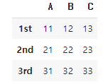
display(df) # HTML로 출력👉 결과
2.3 데이터 추가 하기와 삭제하기
행 추가하기
	df = pd.DataFrame({'A':[11,21,31], 'B':[12,22,32], 'C':[13,23,33]}
                  , index=['1st','2nd','3rd'])
    df.loc['4th'] = [41, 42, 43]
    df.loc['8th'] = [81, 82, 83]
    print(df)
결과
A B C
1st 11 12 13
2nd 21 22 23
3rd 31 32 33
4th 41 42 43
8th 81 82 83열 추가하기
	df['D'] = [14, 24, 34, 44, 84]
	print(df)
결과
A B C D
1st 11 12 13 14
2nd 21 22 23 24
3rd 31 32 33 34
4th 41 42 43 44
8th 81 82 83 84열 삭제하기
	df.drop('D', axis = 1, inplace = True) #inplace는 삭제 후 다시 저장
	print(df)
결과
A B C
1st 11 12 13
2nd 21 22 23
3rd 31 32 33
4th 41 42 43
8th 81 82 83행 삭제하기
	df.drop(['4th','8th'], axis = 0, inplace = True) # inplace는 삭제 후 다시 저장
	print(df)
결과
A B C
1st 11 12 13
2nd 21 22 23
3rd 31 32 332.4 인덱싱과 슬라이싱
열선택: df[‘colname’], df.colname, df[[‘colname1’,‘colname2’,‘colname3’]]
	df = pd.DataFrame({'A':[11,21,31], 'B':[12,22,32], 'C':[13,23,33]}
                  , index=['1st','2nd','3rd'])
    print(df['C'])
    print(df[['A','C']])
결과
1st 13
2nd 23
3rd 33
Name: C, dtype: int64
A C
1st 11 13
2nd 21 23
3rd 31 33인덱스 선택: df.loc[], df.loc[[]], df.loc[:], df.loc[:,:]
	print(df.loc['1st']) # 행 선택
	print(df.loc[['1st','3rd']]) # 여러행 선택
결과
A 11
B 12
C 13
Name: 1st, dtype: int64
A B C
1st 11 12 13
3rd 31 32 33 print(df.loc['1st':'2nd']) # 행 슬라이싱
print(df.loc[:,'B':'C']) # 행열 슬라이싱 결과
A B C
1st 11 12 13
2nd 21 22 23
B C
1st 12 13
2nd 22 23
3rd 32 33절대위치선택: df.iloc[], df.iloc[[]], df.iloc[:], df.iloc[:,:]
	print(df.iloc[0]) # 행 선택
	print(df.iloc[[0,2]]) # 여러행 선택
결과
A 11
B 12
C 13
Name: 1st, dtype: int64
A B C
1st 11 12 13
3rd 31 32 33 print(df.iloc[0:3]) # 행 슬라이싱
print(df.iloc[:,1:3]) # 행열 슬라이싱 결과
A B C
1st 11 12 13
2nd 21 22 23
3rd 31 32 33
B C
1st 12 13
2nd 22 23
3rd 32 332.5 탐색하여 슬라이싱
Dataframe의 변수를 이용하여 슬라이싱
	df = pd.DataFrame({'A':[11,21,31], 'B':[12,22,32], 'C':[13,23,33]}
                  , index=['1st','2nd','3rd'])
	print(df[df.C<30]) # 행선택
결과
A B C
1st 11 12 13
2nd 21 22 23 print(df.loc[lambda x: x.C<30]) #행 선택 결과
A B C
1st 11 12 13
2nd 21 22 23 print(df.loc[df['C']<30, ['A','B']]) #행열 선택 결과
A B
1st 11 12
2nd 21 223 데이터프레임 다루기(중급)
3.1 데이터프레임 클래스
- Python의 모든 자료구조는 클래스(class)임
- 클래스는 객체로서 변수와 메소드(함수)의 집합체 - 따라서 데이터프레임 객체의 변수와 메소드는 직접 사용이 가능함
데이터프레임의 변수와 메서드 보기
	df = pd.DataFrame({'A':[11,21,31], 'B':[12,22,32], 'C':[13,23,33]},
                  index=['1st','2nd','3rd'])
	print(dir(df)[:20])
결과
['A', 'B', 'C', 'T', '_AXIS_LEN', '_AXIS_ORDERS', '_AXIS_TO_AXIS_NUMBER', '_HANDLED_TYPES', '__abs__', '__add__', '__and__', '__annotations__', '__array__', '__array_priority__', '__array_ufunc__', '__bool__', '__class__', '__contains__', '__copy__', '__dataframe__']3.2 데이터프레임 변수
데이터프레임의 열
	df = pd.DataFrame({'A':[11,21,31], 'B':[12,22,32], 'C':[13,23,33]},
                  index=['1st','2nd','3rd'])
	print(df.A) # .컬럼명
결과
1st 11
2nd 21
3rd 31
Name: A, dtype: int64데이터프레임의 T(transpose, 전치행렬)
- 전치행렬이 이미 클래스 내의 T변수에 저장이 되어 있으므로 별도로 계산할 필요없이 바로 사용하면 됨
print(df.T) # .T transpose 결과
1st 2nd 3rd
A 11 21 31
B 12 22 32
C 13 23 333.3 사칙연산
	df1 = pd.DataFrame({'A':[11,21,31], 'B':[12,22,32], 'C':[13,23,33]}
                  , index=['1st','2nd','3rd'])
    df2 = pd.DataFrame({'A':[11,21,41], 'B':[12,22,42], 'E':[14,24,44]}
                      , index=['1st','2nd','4th'])

	print(df1+df2)  # 각 원소별 매칭되는 것만 더하기
결과
A B C E
1st 22.0 24.0 NaN NaN
2nd 42.0 44.0 NaN NaN
3rd NaN NaN NaN NaN
4th NaN NaN NaN NaN print(df1.add(df2, fill_value=0)) # 값이 없는 것은 0으로 대체하여 각 원소별 더하기 결과
A B C E
1st 22.0 24.0 13.0 14.0
2nd 42.0 44.0 23.0 24.0
3rd 31.0 32.0 33.0 NaN
4th 41.0 42.0 NaN 44.0 print(df1.mul(df2, fill_value=1)) # 값이 없는 것은 1로 대체하여 각 원소별 더하기 결과
A B C E
1st 121.0 144.0 13.0 14.0
2nd 441.0 484.0 23.0 24.0
3rd 31.0 32.0 33.0 NaN
4th 41.0 42.0 NaN 44.03.4 Assign
- 기존의 열을 이용하여 새로운 열을 생성
	df = pd.DataFrame({'A':[11,21,31], 'B':[12,22,32], 'C':[13,23,33]}
                  , index=['1st','2nd','3rd'])
	print(df)
결과
A B C
1st 11 12 13
2nd 21 22 23
3rd 31 32 33새로운 열 생성
print(df.assign(A_plus_B = df.A+df.B)) 결과
A B C A_plus_B
1st 11 12 13 23
2nd 21 22 23 43
3rd 31 32 33 63새로운 열 생성(callable)
    import numpy as np
    print(df.assign(log_A = lambda x:np.log(x.A)))
결과
A B C log_A
1st 11 12 13 2.397895
2nd 21 22 23 3.044522
3rd 31 32 33 3.4339873.5 열 수정
	df = pd.DataFrame({'A':[11,21,31], 'B':[12,22,32], 'C':[13,23,33]}
                  , index=['1st','2nd','3rd'])
    df.insert(loc=0, column='D', value=[14,24,34])  # 열 삽입, df자체가 변경됨
    df.insert(loc=2, column='E', value=5)  # 열 삽입
    print(df)
결과
D A E B C
1st 14 11 5 12 13
2nd 24 21 5 22 23
3rd 34 31 5 32 33 df = df.drop(columns = ['D','E']) # 열 제거, df에 저장해 주어야 함
print(df) 결과
A B C
1st 11 12 13
2nd 21 22 23
3rd 31 32 33 df = df.rename(columns = {'A':'aaa'}) # 열이름 변경
print(df) 결과
aaa B C
1st 11 12 13
2nd 21 22 23
3rd 31 32 333.6 값 수정
	df = pd.DataFrame({'A':[11,21,31], 'B':[12,22,32], 'C':[13,23,33]}
                  , index=['1st','2nd','3rd'])
	print(df)
결과
A B C
1st 11 12 13
2nd 21 22 23
3rd 31 32 33위치지정 수정
	df['2nd','A'] = 201  # 잘못된 명령어
	print(df)
결과
A B C (2nd, A)
1st 11 12 13 201
2nd 21 22 23 201
3rd 31 32 33 201 df.loc['2nd','A'] = 222
print(df) 결과
A B C (2nd, A)
1st 11 12 13 201
2nd 222 22 23 201
3rd 31 32 33 201 df.iloc[:,3] = 'NA'
print(df) 결과
A B C (2nd, A)
1st 11 12 13 NA
2nd 222 22 23 NA
3rd 31 32 33 NA값을 찾아서 대체
	df = df.replace('NA', 1111)
	print(df)
결과
A B C (2nd, A)
1st 11 12 13 1111
2nd 222 22 23 1111
3rd 31 32 33 1111 df = df.replace({'B':32}, 9999)
print(df) 결과
A B C (2nd, A)
1st 11 12 13 1111
2nd 222 22 23 1111
3rd 31 9999 33 11113.7 데이터 정렬
	df = pd.DataFrame({'A':[11,21,31], 'B':[12,22,32], 'C':[33,32,31]}
                  , index=['1st','2nd','3rd'])
	print(df)
결과
A B C
1st 11 12 33
2nd 21 22 32
3rd 31 32 31정렬
	df = df.sort_values(by='A', ascending=False) # 값기준 정렬
	print(df)
결과
A B C
3rd 31 32 31
2nd 21 22 32
1st 11 12 33 df = df.sort_index(axis=0) # 행 index 정렬
print(df) 결과
A B C
1st 11 12 33
2nd 21 22 32
3rd 31 32 31랭크
	df_rank = df.rank(axis=0, method='average', ascending=False)   # 열기준, 평균순위, 역순
	print(df_rank)
결과
A B C
1st 3.0 3.0 1.0
2nd 2.0 2.0 2.0
3rd 1.0 1.0 3.03.8 Melt
- pandas.melt()를 이용하여 wide format 데이터를 column format으로 변경
- id_var: 식별자 변수
- value_vars: 해체할 열
- var_name: 변수에 사용할 열이름
- value_name: 해체된 열에 사용할 열이름
- col_level: multiindex인 경우 이 수준을 사용
	df = pd.DataFrame({'order': ['1st','2nd','3rd'],'A':[11,21,31], 'B':[12,22,32], 'C':[33,32,31]})
	print(df)
결과
order A B C
0 1st 11 12 33
1 2nd 21 22 32
2 3rd 31 32 31 df_melted = pd.melt(df, id_vars=['order'], value_vars=['A','B','C'], var_name='name', value_name='score')
print(df_melted) 결과
order name score
0 1st A 11
1 2nd A 21
2 3rd A 31
3 1st B 12
4 2nd B 22
5 3rd B 32
6 1st C 33
7 2nd C 32
8 3rd C 313.9 통계 처리
산술통계량 계산
- axis=0: 열별, axis=1: 행별, ddof=1: 표본 자유도 반영
print(df.count(axis=0)) # 데이터 갯수 결과
order 3
A 3
B 3
C 3
dtype: int64- 최근 파이썬 버전부터는 수치형이 아닌경우 오류가 발생
	df_numeric = df[['A','B','C']]

	df_numeric.mean(axis=1) # 평균
결과
0 18.666667
1 25.000000
2 31.333333
dtype: float64 df_numeric.max(axis=0) # 최대값 결과
A 31
B 32
C 33
dtype: int64 df_numeric.var(axis=1, ddof=1) # 표본분산 결과
0 154.333333
1 37.000000
2 0.333333
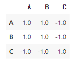
dtype: float64 df_numeric.corr() # 상관계수👉 결과
기술통계량 요약
	df = pd.DataFrame({'A':[11,21,31,41], 'B':[12,22,32,42], 'C':[13,23,33,43]}
                  , index=['1st','2nd','3rd','4th'])
	print(df.describe()) #기술통계량
결과
A B C
count 4.000000 4.000000 4.000000
mean 26.000000 27.000000 28.000000
std 12.909944 12.909944 12.909944
min 11.000000 12.000000 13.000000
25% 18.500000 19.500000 20.500000
50% 26.000000 27.000000 28.000000
75% 33.500000 34.500000 35.500000
max 41.000000 42.000000 43.000000샘플링
print(df.sample(n=2)) 결과
A B C
1st 11 12 13
2nd 21 22 23 print(df.sample(frac=0.5)) 결과
A B C
2nd 21 22 23
1st 11 12 133.10 데이터 정제
	df = pd.DataFrame({'A':[11,21,31,None,31], 'B':[12,22,32,42,32], 'C':[13,None,33,43,33]}
                  , index=['1st','2nd','3rd','4th','7th'])
	print(df)
결과
A B C
1st 11.0 12 13.0
2nd 21.0 22 NaN
3rd 31.0 32 33.0
4th NaN 42 43.0
7th 31.0 32 33.0중복데이터 제거
print(df.drop_duplicates()) 결과
A B C
1st 11.0 12 13.0
2nd 21.0 22 NaN
3rd 31.0 32 33.0
4th NaN 42 43.0결측치 행 제거
- 결측값 있는 행 제거 : df.dropna() or df.dropna(axis=0)
- 결측값 있는 열 제거 : df.dropna(axis=1)
print(df.dropna()) 결과
A B C
1st 11.0 12 13.0
3rd 31.0 32 33.0
7th 31.0 32 33.0결측치 대체
- 결측값을 특정 값으로 채우기 : df.fillna(특정값)
- 결측값을 결측값의 앞 행의 값으로 채우기 : df.fillna(method=‘ffill’) or df.fillna(method=‘pad’)
- 결측값을 결측값의 뒷 행의 값으로 채우기 : df.fillna(method=‘bfill’) or df.fillna(method=‘backfill’)
- 결측값을 각 열의 평균 값으로 채우기 : df.fillna(df.mean())
print(df) 결과
A B C
1st 11.0 12 13.0
2nd 21.0 22 NaN
3rd 31.0 32 33.0
4th NaN 42 43.0
7th 31.0 32 33.0 print(df.fillna(axis=1, method='ffill')) 결과
A B C
1st 11.0 12.0 13.0
2nd 21.0 22.0 22.0
3rd 31.0 32.0 33.0
4th NaN 42.0 43.0
7th 31.0 32.0 33.0 print(df.fillna(df.mean())) 결과
A B C
1st 11.0 12 13.0
2nd 21.0 22 30.5
3rd 31.0 32 33.0
4th 23.5 42 43.0
7th 31.0 32 33.03.11 filter
- 데이터를 필터링하는 유용한 함수
- 람다함수와 정규표현식(regex) 사용이 가능하여 데이터 전처리시 유용
	df = pd.DataFrame({'abc':[1,4,7], 'bcd':[2,5,8], 'abd':[3,6,9]}, index=['1st','2nd','3rd'])
	print(df)
결과
abc bcd abd
1st 1 2 3
2nd 4 5 6
3rd 7 8 9컬럼명으로 선택
print(df.filter(items=['abc', 'abd'])) 결과
abc abd
1st 1 3
2nd 4 6
3rd 7 9정규표현식으로 선택
print(df.filter(regex='^ab', axis=1)) # 열이름이 ab로 시작하는 열 선택 결과
abc abd
1st 1 3
2nd 4 6
3rd 7 9문자열 포함으로 선택
print(df.filter(like='d', axis=0)) # 인덱스명에 d가 포함된 행 선택 결과
abc bcd abd
2nd 4 5 6
3rd 7 8 93.12 Query
- 조건에 부합하는 데이터를 추출할 때 가장 많이 사용
- .loc[ ] 로 구현한 것보다 속도가 느림
	df = pd.DataFrame({'abc':[1,4,7], 'bcd':[2,5,8], 'abd':[3,6,9]}, index=['1st','2nd','3rd'])
	print(df)
결과
abc bcd abd
1st 1 2 3
2nd 4 5 6
3rd 7 8 9질의어로 선택
print(df.query('abc > 3')) 결과
abc bcd abd
2nd 4 5 6
3rd 7 8 9 print(df.query('(abc > 3) & (abd < 9)')) 결과
abc bcd abd
2nd 4 5 6외부 값(함수) 참조 @
	abd_max = 9
	print(df.query('(abc > 3) & (abd < @abd_max)'))
결과
abc bcd abd
2nd 4 5 63.13 Groupby
- 범주별로 그룹을 만들어서 데이터를 처리하고 Series로 반환
	df = pd.DataFrame({'scale':['small','large','small','large']
                   , 'location':['east','east','south','south'], 'sales':[10,20,30,40]})
	print(df)
결과
scale location sales
0 small east 10
1 large east 20
2 small south 30
3 large south 40scale별로 그룹을 나누어 sales의 합계를 구함
	data_s = df.groupby(by='scale')['sales'].sum()
    print(data_s)
    print(type(data_s))  # Series 데이터
    print(data_s.index)
    print(data_s.values)
결과
scale
large 60
small 40
Name: sales, dtype: int64
<class 'pandas.core.series.Series'>
Index(['large', 'small'], dtype='object', name='scale')
[60 40]location-scale별로 그룹을 나누어 sales의 평균을 구함
	data_sl = df.groupby(by=['location', 'scale'])['sales'].mean()
    print(data_sl)
    print(type(data_sl))  # Series 데이터
    print(data_sl.index)
    print(data_sl.values)
결과
location scale
east large 20.0
small 10.0
south large 40.0
small 30.0
Name: sales, dtype: float64
<class 'pandas.core.series.Series'>
MultiIndex([( 'east', 'large'),
( 'east', 'small'),
('south', 'large'),
('south', 'small')],
names=['location', 'scale'])
[20. 10. 40. 30.]location-scale별로 그룹을 나누어 sales의 평균을 구하여 데이터프레임으로 반환
	data_sl = df.groupby(by=['location', 'scale'])[['sales']].mean()
    print(data_sl)
    print(type(data_sl))  # Series 데이터
    print(data_sl.index)
    print(data_sl.values)
결과
sales
location scale
east large 20.0
small 10.0
south large 40.0
small 30.0
<class 'pandas.core.frame.DataFrame'>
MultiIndex([( 'east', 'large'),
( 'east', 'small'),
('south', 'large'),
('south', 'small')],
names=['location', 'scale'])
[[20.]
[10.]
[40.]
[30.]]3.14 Apply
- 객체(함수)를 반복하여 적용
- 파이썬 내장함수 map과 유사
	df = pd.DataFrame({'scale':['small','large','small','large']
                   , 'location':['east','east','south','south'], 'sales':[10,20,30,40]})
	print(df)
결과
scale location sales
0 small east 10
1 large east 20
2 small south 30
3 large south 40map 적용
print(list(map(lambda x: x**2, df.sales))) 결과
[100, 400, 900, 1600]apply 적용
print(df.sales.apply(lambda x: x**2)) 결과
0 100
1 400
2 900
3 1600
Name: sales, dtype: int643.15 Join
	df1 = pd.DataFrame({'id':['1st','2nd','3rd'], 'name': ['홍길동', '임꺽정', '김홍익']})
    df2 = pd.DataFrame({'id':['2nd','3rd','4th'], 'address': ['서울', '강원도', '경기도']})
    print(df1)
    print(df2)
결과
id name
0 1st 홍길동
1 2nd 임꺽정
2 3rd 김홍익
id address
0 2nd 서울
1 3rd 강원도
2 4th 경기도합치기(Concat) -> axis = 0: 행으로 합침, axis = 1: 열로 합침
	concat_row = pd.concat([df1,df2], axis = 0)
    concat_col = pd.concat([df1,df2], axis = 1)

    print('행으로 합침: \n', concat_row)
    print('열로 합침: \n', concat_col)
결과
행으로 합침:
id name address
0 1st 홍길동 NaN
1 2nd 임꺽정 NaN
2 3rd 김홍익 NaN
0 2nd NaN 서울
1 3rd NaN 강원도
2 4th NaN 경기도
열로 합침:
id name id address
0 1st 홍길동 2nd 서울
1 2nd 임꺽정 3rd 강원도
2 3rd 김홍익 4th 경기도조인(Join)
- 내부 결합(Inner Join): 두 개의 테이블 키가 일치하는 데이터만 추출
- 외부 결합(Outer Join): 두 개의 테이블 키와 관련된 모든 데이터 추출
	inner_join = pd.merge(df1, df2, on='id', how='inner')
    outer_join = pd.merge(df1, df2, on='id', how='outer')
    print('inner: \n', inner_join)
    print('outer: \n', outer_join)
결과
inner:
id name address
0 2nd 임꺽정 서울
1 3rd 김홍익 강원도
outer:
id name address
0 1st 홍길동 NaN
1 2nd 임꺽정 서울
2 3rd 김홍익 강원도
3 4th NaN 경기도- 좌 결합(Left Join): 왼쪽 테이블 키와 일치하는 데이터 추출
- 우 결합(Right Join): 오른쪽 테이블 키와 일치하는 데이터 추출
	left_join = pd.merge(df1, df2, on='id', how='left')
    right_join = pd.merge(df1, df2, on='id', how='right')
    print('left: \n', left_join)
    print('right: \n', right_join)
결과
left:
id name address
0 1st 홍길동 NaN
1 2nd 임꺽정 서울
2 3rd 김홍익 강원도
right:
id name address
0 2nd 임꺽정 서울
1 3rd 김홍익 강원도
2 4th NaN 경기도4 데이터프레임 다루기(고급)
4.1 메서드 결합
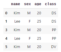
	df = pd.DataFrame({'name':['Kim','Lee','Park','Kim','Lee','Kim']
                   , 'sex':['M','F','F','M','F','M']
                   , 'age':[20,25,30,20,25,20]
                   , 'class':['DS','DS','DS','PP','PP','DV']})
	print(df)
결과
name sex age class
0 Kim M 20 DS
1 Lee F 25 DS
2 Park F 30 DS
3 Kim M 20 PP
4 Lee F 25 PP
5 Kim M 20 DVclass 별 수강학생수
df.groupby(by='class')['name'].count() 결과
class
DS 3
DV 1
PP 2
Name: name, dtype: int64학생별 수강교과목의 갯수
df.groupby(by=['name','sex','age'])['class'].count() 결과
name sex age
Kim M 20 3
Lee F 25 2
Park F 30 1
Name: class, dtype: int64학생별 수강교과목이 2개 이상인 데이터만 필터링
df.groupby(by=['name','sex','age']).filter(lambda x: len(x)>=2)👉 결과
2 class 이상 수강하는 학생의 이름
df.groupby(by=['name','sex','age']).filter(lambda x: len(x)>=2)['name'].unique() 결과
array(['Kim', 'Lee'], dtype=object)2 class 이상 수강하는 학생의 평균 나이
	(df
      .groupby(by=['name','sex','age'])
      .filter(lambda x: len(x)>=2)[['name','age']]
      .drop_duplicates()['age']
      .mean())
결과
22.54.2 Pandas 그래프
- 판다스는 Matplotlib 라이브러리의 기능을 일부 내장하고 있어 간단한 그래프를 그릴 수 있음
- 판다스에서 제공하는 plot(kind='옵션’) 메소드를 이용하여 그림
- ‘line’ : line plot (default)
- ‘bar’ : vertical bar plot
- ‘barh’ : horizontal bar plot
- ‘hist’ : histogram
- ‘box’ : boxplot
- ‘kde’ : Kernel Density Estimation plot
- ‘density’ : same as ‘kde’
- ‘area’ : area plot
- ‘pie’ : pie plot
- scatter’ : scatter plot (DataFrame only)
- ‘hexbin’ : hexbin plot (DataFrame only)
import pandas as pd
import matplotlib.pyplot as plt
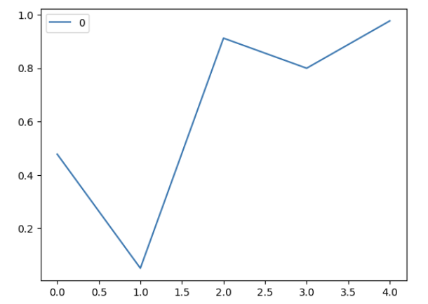
df1 = pd.DataFrame(np.random.rand(5))
print(df1.head())
df2 = pd.DataFrame(np.random.rand(5))
print(df2.head()) 결과
0
0 0.603505
1 0.638853
2 0.686185
3 0.773065
4 0.742881
0
0 0.401318
1 0.021973
2 0.496399
3 0.966737
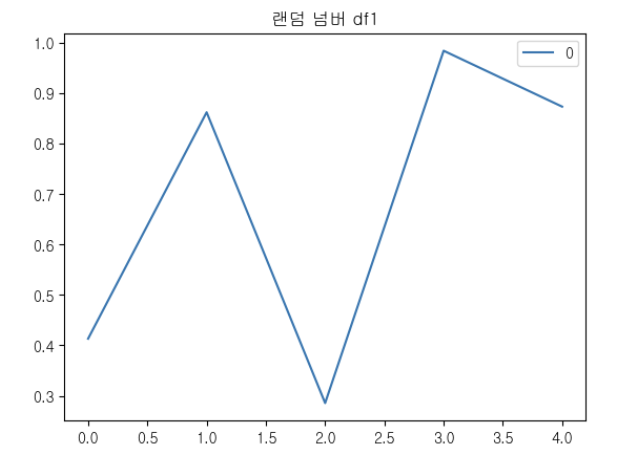
4 0.949217 df1.plot()
df2.plot()
plt.title("랜덤 넘버 df1")
plt.rc('font', family='gulim')
plt.show()👉 결과1
👉 결과2
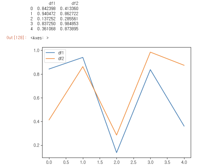
	df = pd.concat([df1,df2], axis=1)
    df.columns = ['df1', 'df2']
    print(df.head())
    df.plot()
👉 결과
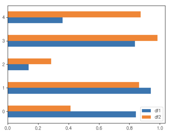
df.plot(kind='barh')👉 결과
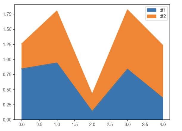
df.plot(kind='area')👉 결과
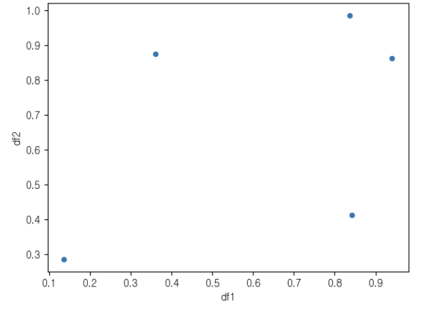
df.plot(kind='scatter', x='df1', y='df2')👉 결과
5 다양한 그래프 그려보기
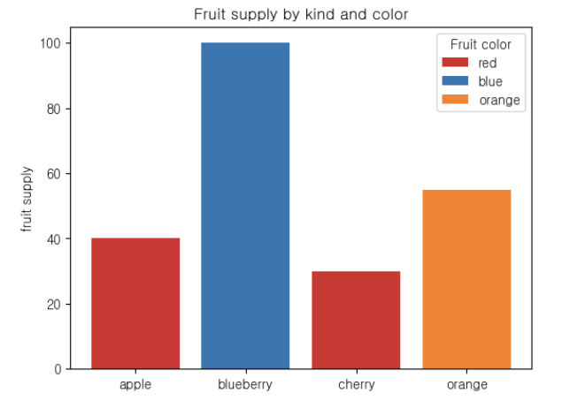
- 아래 그래프가 출력될 수 있도록 코드를 작성해보자
	import matplotlib.pyplot as plt

    fig, ax = plt.subplots()

    fruits = ['apple', 'blueberry', 'cherry', 'orange']
    counts = [40, 100, 30, 55]
    bar_labels = ['red', 'blue', '_red', 'orange']
    bar_colors = ['tab:red', 'tab:blue', 'tab:red', 'tab:orange']

    ax.bar(fruits, counts, label=bar_labels, color=bar_colors)

    ax.set_ylabel('fruit supply')
    ax.set_title('Fruit supply by kind and color')
    ax.legend(title='Fruit color')

    plt.show()
👉 결과
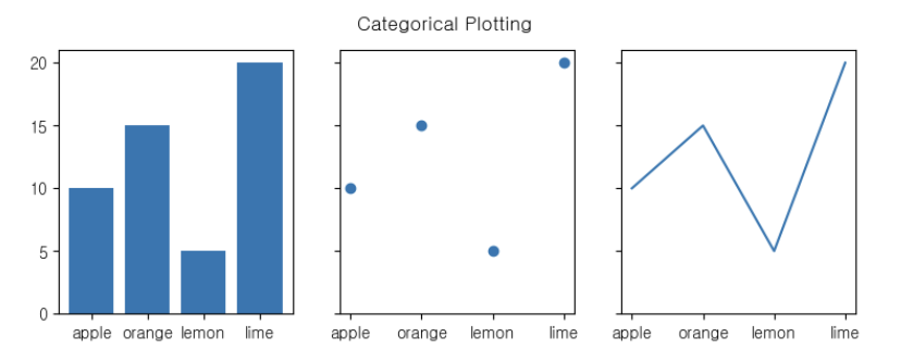
	import matplotlib.pyplot as plt

    data = {'apple': 10, 'orange': 15, 'lemon': 5, 'lime': 20}
    names = list(data.keys())
    values = list(data.values())

    fig, axs = plt.subplots(1, 3, figsize=(9, 3), sharey=True)
    axs[0].bar(names, values)
    axs[1].scatter(names, values)
    axs[2].plot(names, values)
    fig.suptitle('Categorical Plotting')
👉 결과
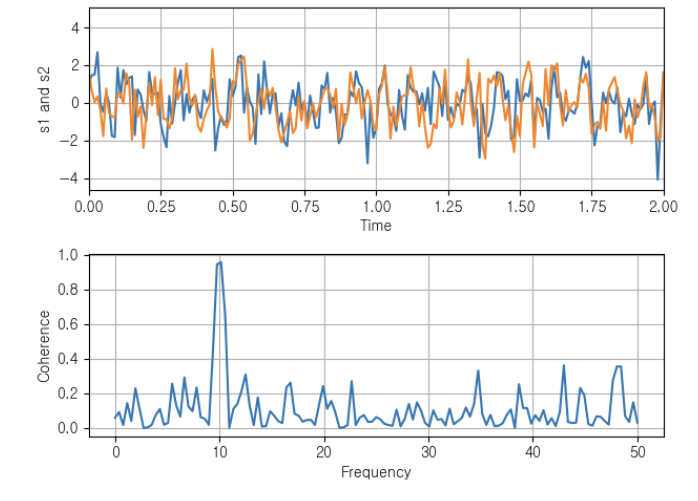
	import numpy as np
    import matplotlib.pyplot as plt

    # Fixing random state for reproducibility
    np.random.seed(19680801)

    dt = 0.01
    t = np.arange(0, 30, dt)
    nse1 = np.random.randn(len(t))                 # white noise 1
    nse2 = np.random.randn(len(t))                 # white noise 2

    # Two signals with a coherent part at 10 Hz and a random part
    s1 = np.sin(2 * np.pi * 10 * t) + nse1
    s2 = np.sin(2 * np.pi * 10 * t) + nse2

    fig, axs = plt.subplots(2, 1)
    axs[0].plot(t, s1, t, s2)
    axs[0].set_xlim(0, 2)
    axs[0].set_xlabel('Time')
    axs[0].set_ylabel('s1 and s2')
    axs[0].grid(True)

    cxy, f = axs[1].cohere(s1, s2, 256, 1. / dt)
    axs[1].set_ylabel('Coherence')

    fig.tight_layout()
    plt.show()
👉 결과
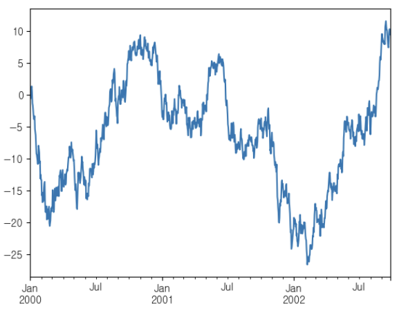
	import matplotlib.pyplot as plt
    import pandas as pd

    ts = pd.Series(np.random.randn(1000), index=pd.date_range("1/1/2000", periods=1000))
    ts = ts.cumsum()
    ts.plot()
👉 결과
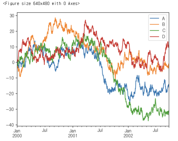
	df = pd.DataFrame(np.random.randn(1000, 4), index=ts.index, columns=list("ABCD"))
    df = df.cumsum()
    plt.figure()
    df.plot()
👉 결과
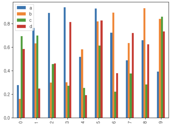
	df2 = pd.DataFrame(np.random.rand(10, 4), columns=["a", "b", "c", "d"])
	df2.plot.bar()
👉 결과
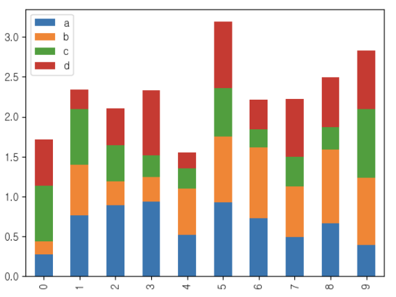
df2.plot.bar(stacked=True)👉 결과
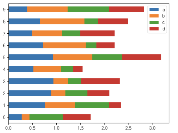
df2.plot.barh(stacked=True)👉 결과
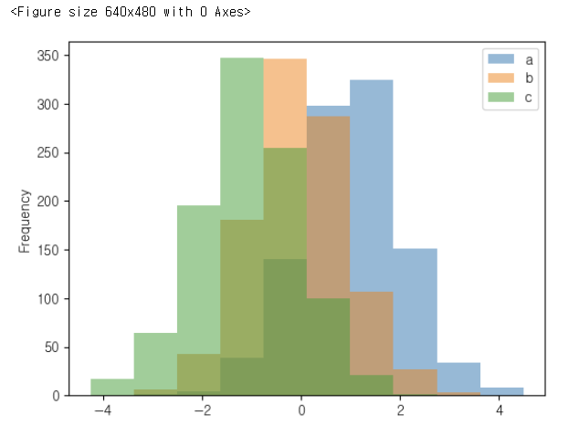
	df4 = pd.DataFrame(
    {
        "a": np.random.randn(1000) + 1,
        "b": np.random.randn(1000),
        "c": np.random.randn(1000) - 1,
    },
    columns=["a", "b", "c"],
)
    plt.figure()
    df4.plot.hist(alpha=0.5)
👉 결과
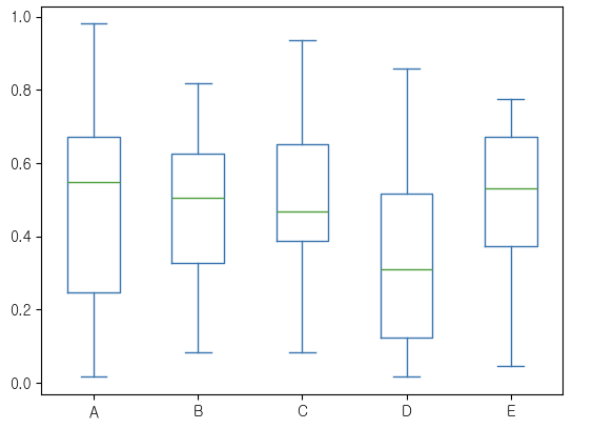
	df = pd.DataFrame(np.random.rand(10, 5), columns=["A", "B", "C", "D", "E"])
	df.plot.box()
👉 결과

나의 기록장