차원 축소(Dimensionality Reduction)
차원 축소(Dimensionality Reduction)는 고차원 데이터에서 중요한 정보는 유지하면서, 데이터의 차원을 줄이는 과정입니다. 이는 주로 데이터의 복잡성을 줄이고, 계산 비용을 절감하며, 노이즈를 줄이고, 시각화를 용이하게 하기 위해 사용됩니다. 차원 축소는 머신 러닝, 데이터 시각화, 데이터 전처리 등 다양한 분야에서 중요한 역할을 합니다.
차원 축소의 필요성
차원 축소(Dimensionality Reduction)는 데이터 분석, 머신 러닝, 데이터 시각화 등 다양한 분야에서 매우 중요한 역할을 합니다. 데이터의 차원이 증가할수록 분석의 복잡성이 기하급수적으로 증가하므로, 이를 효과적으로 관리하고 분석하기 위해 차원 축소가 필요합니다. 차원 축소는 다음과 같은 이유로 중요합니다.
고차원의 저주(Curse of Dimensionality)
고차원의 저주(Curse of Dimensionality)는 데이터의 차원이 증가함에 따라 발생하는 문제들을 지칭하는 용어입니다. 차원이 높아지면, 데이터의 밀도가 희석되고, 데이터 포인트 간의 거리가 급격히 멀어지며, 이는 분석과 모델링을 어렵게 만듭니다.
데이터 스파스티(sparsity)
고차원에서는 데이터 포인트들이 매우 희소하게 분포하게 됩니다. 이는 학습 모델이 유의미한 패턴을 학습하기 어렵게 만듭니다.
거리 기반 알고리즘의 비효율성
차원이 높아지면 데이터 포인트 간의 거리가 거의 같아져서, K-최근접 이웃(K-NN)이나 군집화(clustering)와 같은 거리 기반 알고리즘의 성능이 저하됩니다.
연산 복잡도 증가
차원이 증가함에 따라, 연산의 복잡도도 지수적으로 증가 합니다. 이는 모델 훈련과 예측에 더 많은 시간이 소요됨을 의미합니다.
계산 비용 절감
차원이 높은 데이터는 처리하는 데 많은 연산 자원을 필요로 합니다. 차원 축소를 통해 데이터의 차원을 줄이면, 계산 비용이 크게 감소합니다. 이는 특히 대규모 데이터셋을 다루는 빅데이터 분석에서 매우 중요합니다.
메모리 사용량 감소
차원이 줄어들면, 데이터를 저장하고 처리하는데 필요한 메모리 사용량이 줄어듭니다.
모델 훈련 시간 단축
차원 축소를 통해 피처 수를 줄이면, 모델 훈련에 필요한 시간이 단축됩니다. 이는 실시간 애플리케이션이나 대규모 데이터셋을 처리할 때 유리합니다.
모델 예측 시간 단축
모델의 입력 차원이 줄어들면, 예측에 소요되는 시간도 감소합니다.
import numpy as np

np.random.seed(4)
m = 60
w1, w2 = 0.1, 0.3
noise = 0.1

angles = np.random.rand(m) * 3 * np.pi / 2 - 0.5
x = np.empty((m,3))     # 3차원 안에 m개의 데이터
x[:, 0] = np.cos(angles) * np.sin(angles) / 2 + noise * np.random.rand(m) / 2
x[:, 1] = np.sin(angles) * 0.7 + noise * np.random.randn(m) / 2
x[:, 2] = x[:, 0] * w1 + x[:,1] * w2 + noise * np.random.randn(m)
print(x)
print(x.shape)

x_centered = x - x.mean(axis=0)
print(x_centered)
print()

u, s, Vt = np.linalg.svd(x_centered)
print()

print(u.shape)
print(s.shape)
print(Vt.shape)
W2 = Vt.T[:, :2]
print(W2)
print()

x2d = x_centered.dot(W2)
print(x2d)
print(x2d.shape)
print()

from sklearn.decomposition import PCA
pca = PCA(n_components=3)
x2d2 = pca.fit_transform(x)
print(x2d2)
print()
print(pca.explained_variance_ratio_)
print()
cumsum = np.cumsum(pca.explained_variance_ratio_)
print(cumsum)
d = np.argmax(cumsum >= 0.95) + 1
[[ 0.28682703 -0.47603279 -0.12606828]
 [-0.19225406  0.60125285  0.05666808]
 [ 0.2543851  -0.56464252 -0.10789045]
 [-0.10125473  0.1719946  -0.11001752]
 [-0.12016352  0.24647244  0.06744314]
 [ 0.25821967  0.33475532 -0.01777793]
 [ 0.26486768 -0.4714203  -0.12946399]
 [-0.19784519 -0.2961278  -0.05781553]
 [ 0.27552843  0.36258818  0.3566857 ]
 [ 0.02321394  0.67813799  0.31352622]
 [ 0.05220101 -0.09262183  0.13915767]
 [ 0.2347041   0.33680245  0.13130836]
 [ 0.21361195 -0.22000148  0.16693433]
 [ 0.25902259 -0.60875697 -0.1808507 ]
 [ 0.13268187  0.21879713  0.05368757]
 [-0.22214289  0.50449315  0.00092537]
 [-0.19172826 -0.28888842 -0.08361418]
 [ 0.15019912  0.7650104   0.34988307]
 [-0.11961738 -0.21891348 -0.1410216 ]
 [ 0.28510407 -0.5951168  -0.18708485]
 [ 0.0101773   0.73582959  0.17541211]
 [ 0.25448091 -0.49089286 -0.15496502]
 [ 0.06600822 -0.01093056 -0.05571668]
 [ 0.21864006 -0.24727781 -0.18732331]
 [ 0.17628118  0.18349474  0.21077335]
 [-0.03017093 -0.20070112 -0.26040274]
 [-0.22529412  0.55936443  0.0525717 ]
 [ 0.17816092  0.18077368  0.10642234]
 [-0.06518064  0.06881914  0.11528385]
 [ 0.118327    0.63413304  0.18121253]
 [-0.15178143  0.69645833  0.16543473]
 [ 0.25739772 -0.48156378 -0.11378171]
 [-0.15675091  0.66320805  0.15715612]
 [ 0.04821308  0.04941375  0.10731968]
 [ 0.13543986  0.13635876  0.00616375]
 [-0.20048603  0.55858467  0.04898495]
 [-0.15584713  0.60198613  0.11774484]
 [-0.21941958  0.36107969  0.09600874]
 [ 0.11845028  0.67428648  0.33705231]
 [-0.20725415  0.33875069  0.24088754]
 [ 0.11060749  0.68791584  0.17749407]
 [-0.22586162  0.42768963 -0.04069763]
 [ 0.00831612  0.0136965  -0.13344607]
 [ 0.20363552  0.26816938  0.31334658]
 [ 0.19052794  0.73860522  0.20034738]
 [-0.10888039  0.74708137  0.25902699]
 [-0.17717104  0.28204187  0.25862394]
 [ 0.28261435  0.45912332  0.09798681]
 [-0.18734166  0.57376501  0.13393794]
 [-0.20477331  0.49946905  0.07130387]
 [ 0.24624408 -0.30606478 -0.17678663]
 [ 0.16812412  0.62522819  0.28435642]
 [-0.20850417  0.45465469  0.22211597]
 [ 0.18629396  0.25751291 -0.09149058]
 [-0.09269668  0.66514129  0.28844378]
 [ 0.20447473  0.25564484  0.07354422]
 [ 0.26552589 -0.46357227 -0.09415646]
 [ 0.06511586  0.74430462  0.24958987]
 [ 0.13747018 -0.2618936  -0.19547493]
 [ 0.10011647  0.66124294  0.17729744]]
(60, 3)
[[ 0.24218053 -0.688178   -0.19133855]
 [-0.23690056  0.38910763 -0.0086022 ]
 [ 0.2097386  -0.77678774 -0.17316072]
 [-0.14590123 -0.04015062 -0.1752878 ]
 [-0.16481002  0.03432722  0.00217286]
 [ 0.21357317  0.1226101  -0.0830482 ]
 [ 0.22022118 -0.68356552 -0.19473427]
 [-0.24249169 -0.50827302 -0.12308581]
 [ 0.23088193  0.15044296  0.29141542]
 [-0.02143256  0.46599277  0.24825595]
 [ 0.00755451 -0.30476705  0.0738874 ]
 [ 0.1900576   0.12465723  0.06603809]
 [ 0.16896545 -0.4321467   0.10166406]
 [ 0.21437609 -0.82090219 -0.24612098]
 [ 0.08803537  0.00665191 -0.0115827 ]
 [-0.26678939  0.29234793 -0.0643449 ]
 [-0.23637476 -0.50103364 -0.14888445]
 [ 0.10555262  0.55286518  0.2846128 ]
 [-0.16426388 -0.4310587  -0.20629187]
 [ 0.24045757 -0.80726202 -0.25235513]
 [-0.0344692   0.52368437  0.11014183]
 [ 0.20983441 -0.70303808 -0.2202353 ]
 [ 0.02136172 -0.22307578 -0.12098696]
 [ 0.17399356 -0.45942303 -0.25259359]
 [ 0.13163469 -0.02865048  0.14550308]
 [-0.07481743 -0.41284634 -0.32567301]
 [-0.26994062  0.34721921 -0.01269858]
 [ 0.13351442 -0.03137154  0.04115206]
 [-0.10982714 -0.14332608  0.05001358]
 [ 0.0736805   0.42198782  0.11594225]
 [-0.19642793  0.48431311  0.10016445]
 [ 0.21275122 -0.693709   -0.17905198]
 [-0.20139741  0.45106283  0.09188584]
 [ 0.00356658 -0.16273147  0.0420494 ]
 [ 0.09079336 -0.07578646 -0.05910653]
 [-0.24513253  0.34643945 -0.01628532]
 [-0.20049363  0.38984091  0.05247457]
 [-0.26406608  0.14893447  0.03073847]
 [ 0.07380378  0.46214126  0.27178203]
 [-0.25190065  0.12660547  0.17561727]
 [ 0.06596099  0.47577062  0.1122238 ]
 [-0.27050812  0.21554441 -0.1059679 ]
 [-0.03633038 -0.19844872 -0.19871634]
 [ 0.15898902  0.05602416  0.2480763 ]
 [ 0.14588144  0.52646     0.1350771 ]
 [-0.15352688  0.53493615  0.19375672]
 [-0.22181754  0.06989665  0.19335367]
 [ 0.23796785  0.24697811  0.03271653]
 [-0.23198816  0.36161979  0.06866766]
 [-0.24941981  0.28732383  0.00603359]
 [ 0.20159759 -0.51821    -0.2420569 ]
 [ 0.12347762  0.41308297  0.21908615]
 [-0.25315067  0.24250947  0.15684569]
 [ 0.14164746  0.04536769 -0.15676085]
 [-0.13734318  0.45299607  0.22317351]
 [ 0.15982823  0.04349963  0.00827394]
 [ 0.22087939 -0.67571749 -0.15942674]
 [ 0.02046936  0.5321594   0.18431959]
 [ 0.09282368 -0.47403882 -0.2607452 ]
 [ 0.05546997  0.44909772  0.11202716]]


(60, 60)
(3,)
(3, 3)
[[-0.18607836  0.9474753 ]
 [ 0.93797383  0.09247375]
 [ 0.29254049  0.30616852]]

[[-0.74653179  0.10723982]
 [ 0.40653835 -0.19110891]
 [-0.81829091  0.07387331]
 [-0.06178994 -0.1956183 ]
 [ 0.06350126 -0.1523138 ]
 [ 0.05096876  0.18826677]
 [-0.73911262  0.08582076]
 [-0.46763192 -0.3144418 ]
 [ 0.18340024  0.32188918]
 [ 0.51370207  0.09879343]
 [-0.26565419  0.00159675]
 [ 0.10087843  0.21182119]
 [-0.40704226  0.1512547 ]
 [-0.88187587  0.05184965]
 [-0.01353057  0.08048021]
 [ 0.30503495 -0.24544223]
 [-0.46952695 -0.31587543]
 [ 0.58219278  0.23827349]
 [-0.43410455 -0.25865766]
 [-0.87575869  0.07591387]
 [ 0.52983716  0.04949031]
 [-0.7629047   0.06637124]
 [-0.24860778 -0.03743135]
 [-0.53719707  0.04503382]
 [-0.00880222  0.16661966]
 [-0.4685897  -0.20877594]
 [ 0.37219779 -0.22754132]
 [-0.04223119  0.13620003]
 [-0.09936866 -0.10199982]
 [ 0.41602099  0.14433112]
 [ 0.52012617 -0.11065716]
 [-0.74264924  0.08260657]
 [ 0.48744116 -0.12097505]
 [-0.14100037  0.00120506]
 [-0.10527145  0.06091965]
 [ 0.36580088 -0.20520651]
 [ 0.41831903 -0.13784665]
 [ 0.19782586 -0.22701241]
 [ 0.49925037  0.19587429]
 [ 0.21700104 -0.17319348]
 [ 0.46681648  0.1408521 ]
 [ 0.22151082 -0.26881159]
 [-0.23751198 -0.11361413]
 [ 0.09553714  0.23177209]
 [ 0.50617584  0.22825915]
 [ 0.58700583 -0.03667317]
 [ 0.16340045 -0.14450423]
 [ 0.19694924  0.25832442]
 [ 0.40244595 -0.16533883]
 [ 0.31767893 -0.2079019 ]
 [-0.59439181  0.06897771]
 [ 0.42857607  0.22226861]
 [ 0.32045712 -0.16940704]
 [-0.02966272  0.09040755]
 [ 0.51574234 -0.01991033]
 [ 0.0134814   0.1579891 ]
 [-0.72154497  0.09798018]
 [ 0.54926363  0.12503784]
 [-0.53818701 -0.03571997]
 [ 0.44369263  0.12838536]]
(60, 2)

[[-7.46531787e-01  1.07239823e-01 -6.38165738e-03]
 [ 4.06538347e-01 -1.91108913e-01 -7.61877655e-02]
 [-8.18290910e-01  7.38733086e-02  4.81334880e-02]
 [-6.17899447e-02 -1.95618296e-01 -1.07426897e-01]
 [ 6.35012583e-02 -1.52313797e-01  3.33694445e-02]
 [ 5.09687568e-02  1.88266772e-01 -1.71760144e-01]
 [-7.39112621e-01  8.58207620e-02 -5.28694206e-03]
 [-4.67631921e-01 -3.14441800e-01  1.21410641e-01]
 [ 1.83400238e-01  3.21889177e-01  1.53669145e-01]
 [ 5.13702072e-01  9.87934343e-02  7.47640720e-02]
 [-2.65654194e-01  1.59675106e-03  1.66807294e-01]
 [ 1.00878427e-01  2.11821185e-01 -3.12677636e-02]
 [-4.07042258e-01  1.51254700e-01  1.92546859e-01]
 [-8.81875868e-01  5.18496467e-02 -4.42790679e-03]
 [-1.35305702e-02  8.04802096e-02 -3.56159135e-02]
 [ 3.05034949e-01 -2.45442230e-01 -8.65791431e-02]
 [-4.69526949e-01 -3.15875435e-01  9.40290901e-02]
 [ 5.82192781e-01  2.38273493e-01  4.56400619e-02]
 [-4.34104552e-01 -2.58657659e-01 -1.16875839e-04]
 [-8.75758693e-01  7.59138654e-02 -2.14177918e-02]
 [ 5.29837157e-01  4.94903074e-02 -6.62417579e-02]
 [-7.62904701e-01  6.63712410e-02 -1.91801405e-02]
 [-2.48607782e-01 -3.74313464e-02 -4.06206344e-02]
 [-5.37197065e-01  4.50338217e-02 -1.20573899e-01]
 [-8.80222067e-03  1.66619658e-01  1.07145211e-01]
 [-4.68589705e-01 -2.08775945e-01 -1.37618884e-01]
 [ 3.72197790e-01 -2.27541316e-01 -5.73073083e-02]
 [-4.22311859e-02  1.36200034e-01  1.30323918e-02]
 [-9.93686573e-02 -1.01999822e-01  1.21768754e-01]
 [ 4.16020988e-01  1.44331121e-01 -5.51380761e-02]
 [ 5.20126166e-01 -1.10657156e-01 -1.99950193e-02]
 [-7.42649238e-01  8.26065736e-02  1.42524035e-02]
 [ 4.87441157e-01 -1.20975047e-01 -1.50915827e-02]
 [-1.41000373e-01  1.20506118e-03  9.15415084e-02]
 [-1.05271448e-01  6.09196513e-02 -5.18393893e-02]
 [ 3.65800883e-01 -2.05206514e-01 -6.67492631e-02]
 [ 4.18319034e-01 -1.37846650e-01 -3.05728474e-02]
 [ 1.97825861e-01 -2.27012407e-01  4.67709147e-02]
 [ 4.99250371e-01  1.95874295e-01  7.25902372e-02]
 [ 2.17001036e-01 -1.73193482e-01  1.82315315e-01]
 [ 4.66816480e-01  1.40852097e-01 -7.44699561e-02]
 [ 2.21510823e-01 -2.68811595e-01 -9.76550769e-02]
 [-2.37511983e-01 -1.13614127e-01 -1.04258637e-01]
 [ 9.55371432e-02  2.31772091e-01  1.64658496e-01]
 [ 5.06175845e-01  2.28259150e-01 -9.14938468e-02]
 [ 5.87005828e-01 -3.66731708e-02  3.67163995e-02]
 [ 1.63400447e-01 -1.44504227e-01  2.09506621e-01]
 [ 1.96949242e-01  2.58324425e-01 -1.14789990e-01]
 [ 4.02445946e-01 -1.65338833e-01  1.71922735e-03]
 [ 3.17678935e-01 -2.07901902e-01 -2.56617430e-02]
 [-5.94391811e-01  6.89777055e-02 -9.85656394e-02]
 [ 4.28576071e-01  2.22268606e-01  2.83234703e-02]
 [ 3.20457116e-01 -1.69407037e-01  1.26906152e-01]
 [-2.96627195e-02  9.04075511e-02 -1.94017506e-01]
 [ 5.15742337e-01 -1.99103251e-02  8.65356651e-02]
 [ 1.34813974e-02  1.57989097e-01 -4.86151945e-02]
 [-7.21544968e-01  9.79801842e-02  2.39050572e-02]
 [ 5.49263629e-01  1.25037844e-01 -1.61658872e-02]
 [-5.38187013e-01 -3.57199732e-02 -1.01960383e-01]
 [ 4.43692628e-01  1.28385362e-01 -6.30064573e-02]]

[0.84646045 0.1170002  0.03653935]

[0.84646045 0.96346065 1.        ]
2
출처 : https://wikidocs.net/254641
차원축소 예제 1
import numpy as np
import matplotlib.pyplot as plt
import matplotlib as mpl
from sklearn.model_selection import train_test_split
from sklearn.datasets import fetch_openml
from sklearn.decomposition import PCA
mnist = fetch_openml('mnist_784', as_frame=False, cache=True)
mnist.target = mnist.target.astype(np.uint8)
X = mnist['data']
Y = mnist['target']
X_train, X_test, y_train, y_test = train_test_split(X, Y)
pca = PCA()
pca.fit(X_train)
print(pca.explained_variance_ratio_)
cumsum = np.cumsum(pca.explained_variance_ratio_)
d = np.argmax(cumsum >= 0.95) + 1
print(cumsum)
print('dimention:',d)
# plt.figure(figsize=(6,4))
# plt.plot(cumsum, linewidth=3)
# plt.axis([0,400, 0, 1])
# plt.xlabel('dimentions')
# plt.ylabel('explained variance')
# plt.grid(True)
# plt.show()
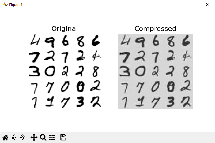
pca = PCA(n_components=154)
X_reduced = pca.fit_transform(X_train)
print(X_reduced.shape)
X_recovered = pca.inverse_transform(X_reduced)
def plot_digits(instances, images_per_row=5, **options):
size = 28
images_per_row = min(len(instances), images_per_row)
images = [instance.reshape(size,size) for instance in instances]
n_rows = (len(instances) - 1) // images_per_row + 1
row_images = []
n_empty = n_rows * images_per_row - len(instances)
images.append(np.zeros((size, size * n_empty)))
for row in range(n_rows):
rimages = images[row * images_per_row : (row + 1) * images_per_row]
row_images.append(np.concatenate(rimages, axis=1))
image = np.concatenate(row_images, axis=0)
plt.imshow(image, cmap = mpl.cm.binary, **options)
plt.axis("off")
plt.figure(figsize=(7, 4))
plt.subplot(121)
plot_digits(X_train[::2100])
plt.title("Original", fontsize=16)
plt.subplot(122)
plot_digits(X_recovered[::2100])
plt.title("Compressed", fontsize=16)
plt.show()
차원축소 예제 2
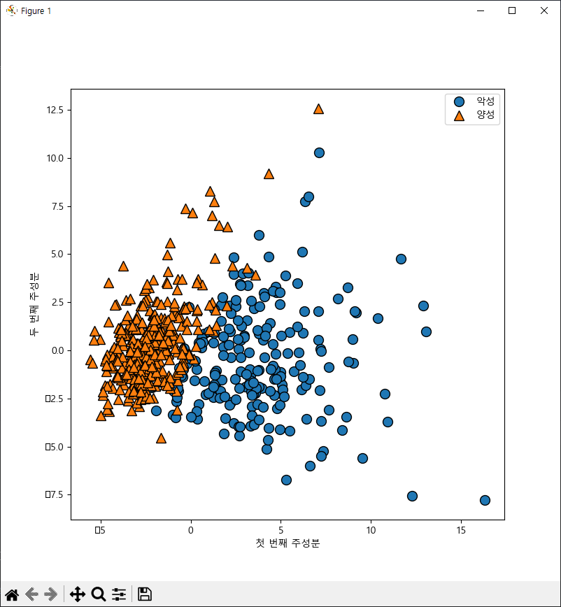
from sklearn.datasets import load_breast_cancer

cancer = load_breast_cancer()
print(cancer.keys())
print(cancer['feature_names'])
print(len(cancer['feature_names']))
print(cancer.data)

from sklearn.preprocessing import StandardScaler
from sklearn.decomposition import PCA
import matplotlib.pyplot as plt
plt.rc('font', family='Malgun Gothic')

scaler = StandardScaler()
x_scaled = scaler.fit_transform(cancer.data)

pca = PCA(n_components=2)
x_pca = pca.fit_transform(x_scaled)
print(x_pca.shape)

import mglearn

plt.figure(figsize=(8,8))
mglearn.discrete_scatter(x_pca[:, 0], x_pca[:, 1], cancer.target)
plt.legend(['악성', '양성'], loc='best')
plt.xlabel('첫 번째 주성분')
plt.ylabel('두 번째 주성분')
plt.show()
차원축소 예제 3
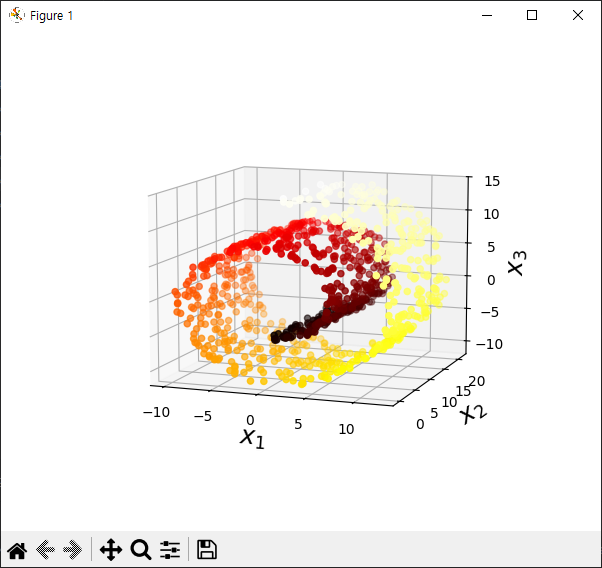
from sklearn.datasets import make_swiss_roll
import matplotlib.pyplot as plt
X, t = make_swiss_roll(n_samples=1000, noise=0.2, random_state=42)
print(X.shape)
print(t.shape)
axes = [-11.5, 14, -2, 23, -12, 15]
fig = plt.figure(figsize=(6, 5))
ax = fig.add_subplot(111, projection='3d')
ax.scatter(X[:, 0], X[:, 1], X[:, 2], c=t, cmap=plt.cm.hot)
ax.view_init(10, -70)
ax.set_xlabel("$x_1$", fontsize=18)
ax.set_ylabel("$x_2$", fontsize=18)
ax.set_zlabel("$x_3$", fontsize=18)
ax.set_xlim(axes[0:2])
ax.set_ylim(axes[2:4])
ax.set_zlim(axes[4:6])
plt.show()
#############################################################
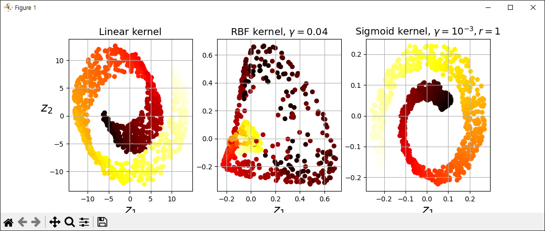
from sklearn.decomposition import KernelPCA
lin_pca = KernelPCA(n_components=2, kernel='linear')
rbf_pca = KernelPCA(n_components=2, kernel='rbf', gamma=0.05)
sig_pca = KernelPCA(n_components=2, kernel='sigmoid', coef0=1, gamma=0.001)
#############################################################
plt.figure(figsize=(11, 4))
for subplot, pca, title in ((131, lin_pca, "Linear kernel"), (132, rbf_pca, "RBF kernel, $\gamma=0.04$"), (133, sig_pca, "Sigmoid kernel, $\gamma=10^{-3}, r=1$")):
X_reduced = pca.fit_transform(X)
if subplot == 132:
X_reduced_rbf = X_reduced
plt.subplot(subplot)
plt.title(title, fontsize=14)
plt.scatter(X_reduced[:, 0], X_reduced[:, 1], c=t, cmap=plt.cm.hot)
plt.xlabel("$z_1$", fontsize=18)
if subplot == 131:
plt.ylabel("$z_2$", fontsize=18, rotation=0)
plt.grid(True)
plt.show()
#하이퍼파라미터 튜닝
#############################################################
from sklearn.pipeline import Pipeline
from sklearn.linear_model import LogisticRegression
import numpy as np
from sklearn.model_selection import GridSearchCV
clf = Pipeline([
('kpca', KernelPCA(n_components=2)),
('log_reg', LogisticRegression())
])
param_grid = [{
'kpca__gamma':np.linspace(0.03, 0.05, 10),
'kpca__kernel':['rbf','sigmoid']
}]
y = t > 6.9
grid_search = GridSearchCV(clf, param_grid, cv=3)
print(grid_search.fit(X, y))
print(grid_search.best_params_)
#############################################################
차원축소 예제 4
from sklearn.datasets import make_swiss_roll
import matplotlib.pyplot as plt
X, t = make_swiss_roll(n_samples=1000, noise=0.2, random_state=42)
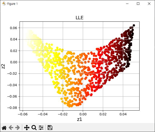
from sklearn.manifold import LocallyLinearEmbedding
lle = LocallyLinearEmbedding(n_components=2, n_neighbors=10, random_state=42)
X_reduced = lle.fit_transform(X)
plt.title('LLE', fontsize=14)
plt.scatter(X_reduced[:, 0], X_reduced[:, 1], c=t, cmap=plt.cm.hot)
plt.xlabel('z1', fontsize=14)
plt.ylabel('z2', fontsize=14)
plt.grid(True)
plt.show()
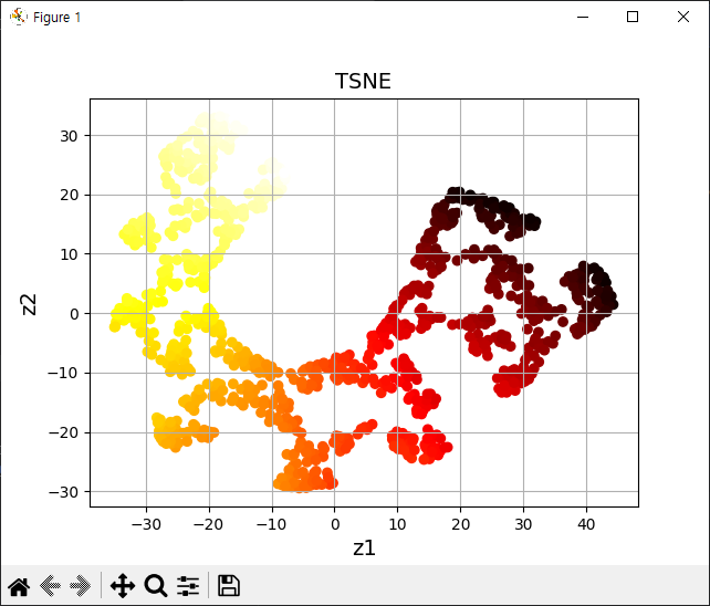
from sklearn.manifold import TSNE
tsne = TSNE(n_components=2, random_state=42)
X_reduced_tsne = tsne.fit_transform(X)
plt.title('TSNE', fontsize=14)
plt.scatter(X_reduced_tsne[:, 0], X_reduced_tsne[:, 1], c=t, cmap=plt.cm.hot)
plt.xlabel('z1', fontsize=14)
plt.ylabel('z2', fontsize=14)
plt.grid(True)
plt.show()
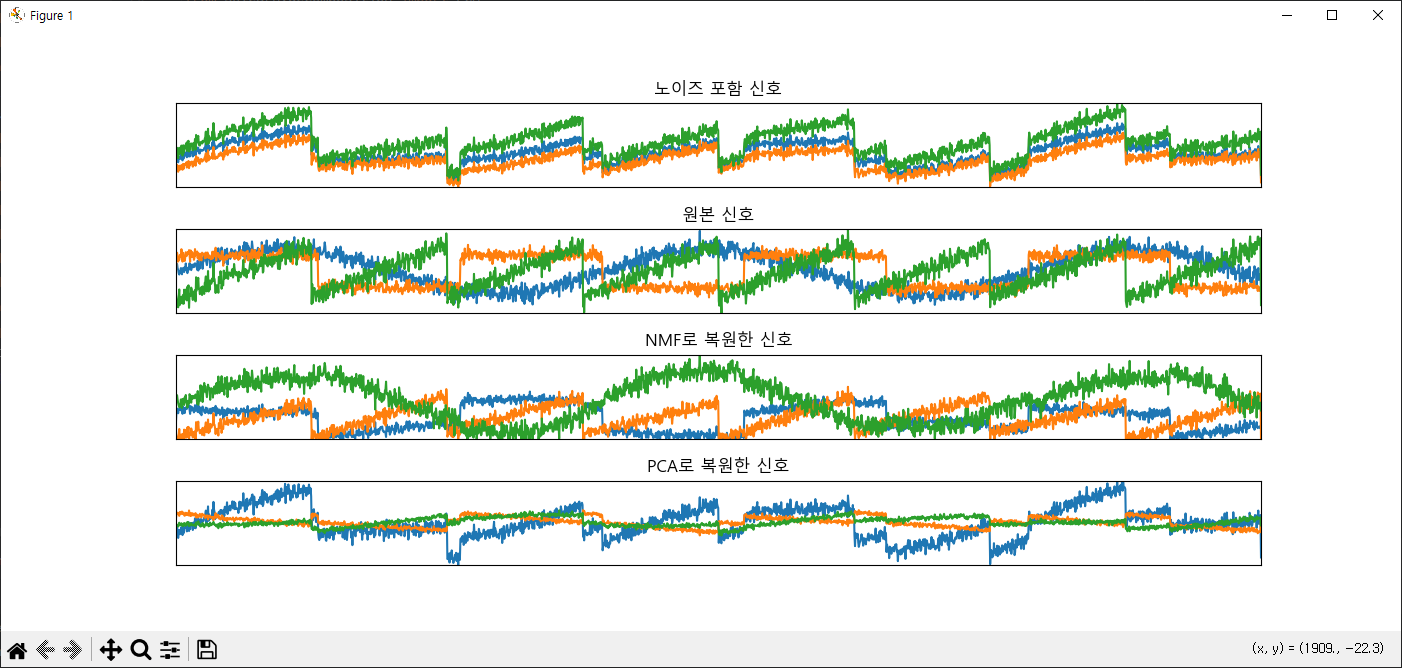
차원축소 예제 5
import mglearn
import matplotlib.pyplot as plt
import numpy as np

plt.rc('font', family='Malgun Gothic')

S = mglearn.datasets.make_signals()
# plt.figure(figsize=(12,3))
# plt.plot(S, '-')
# plt.xlabel('시간')
# plt.ylabel('신호')
# plt.margins(0)
# plt.show()

A = np.random.RandomState(0).uniform(size=(100, 3))
X = np.dot(S, A.T)
print('original signal shape:',S.shape)
print('x shape:', X.shape)

from sklearn.decomposition import PCA
from sklearn.decomposition import NMF

nmf = NMF(n_components=3, random_state=42)
N_S = nmf.fit_transform(X)
print('NS shape:', N_S.shape)

pca = PCA(n_components=3)
P_S = pca.fit_transform(X)

models = [X, S, N_S, P_S]

names = ['노이즈 포함 신호',
         '원본 신호',
         'NMF로 복원한 신호',
         'PCA로 복원한 신호']

fig, axes = plt.subplots(4, figsize=(14,6),
                         gridspec_kw={'hspace':0.5}, subplot_kw={'xticks':(), 'yticks':()})

for model, name, ax in zip(models, names, axes):
    ax.set_title(name)
    ax.plot(model[:, :3], '-')
    ax.margins(0)
plt.show()
차원축소 예제 6
from sklearn.datasets import fetch_openml
import numpy as np
mnist = fetch_openml('mnist_784', as_frame=False)
mnist.target = mnist.target.astype(np.uint8)
np.random.seed(42)
m = 10000
idx = np.random.permutation(60000)[:m]
x = mnist['data'][idx]
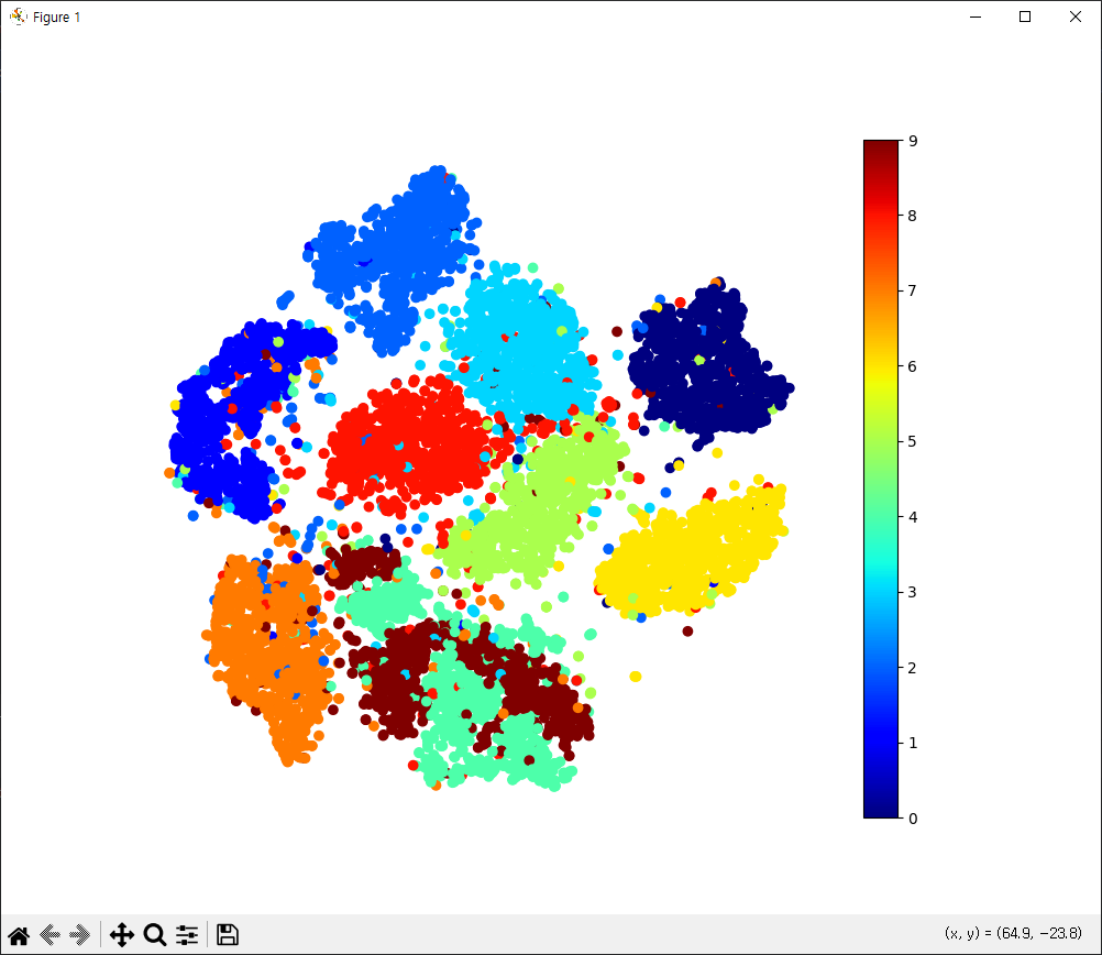
y = mnist['target'][idx] #t-SNE를 이용해서 2차원 축소(특성데이터를)
#2차원 그래프(산점도) 타깃 색깔별로
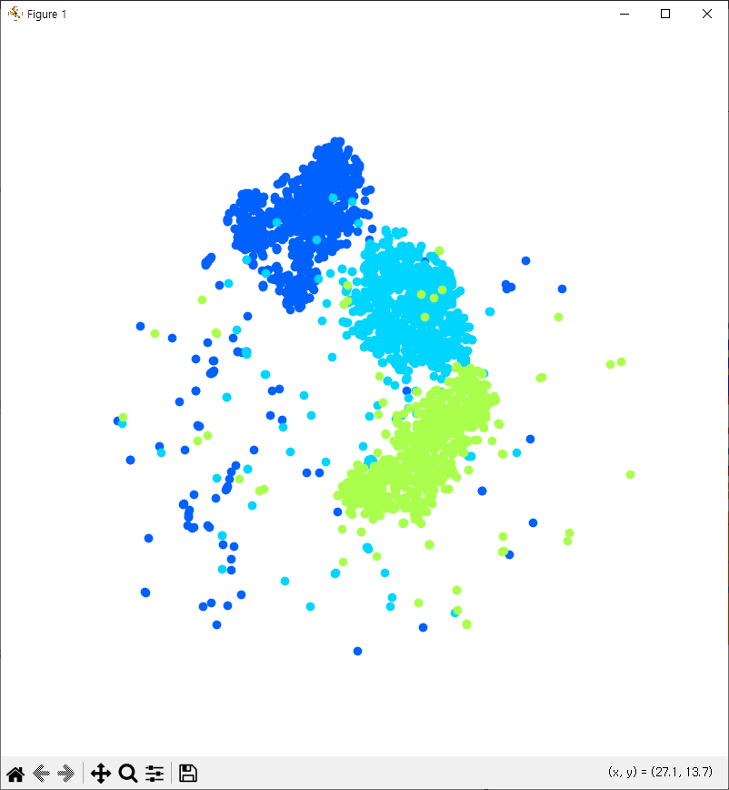
#target 2,3,5, 데이터를 분리를 해서 위의 조건에 맞게 실행
from sklearn.manifold import TSNE
tsne = TSNE(n_components=2, random_state=42)
X_reduced = tsne.fit_transform(x)
import matplotlib.pyplot as plt
plt.figure(figsize=(10,8))
plt.scatter(X_reduced[:, 0], X_reduced[:, 1], c=y, cmap='jet')
plt.axis('off')
plt.colorbar()
plt.show()
import matplotlib as mpl
plt.figure(figsize=(8,8))
cmap = mpl.cm.get_cmap('jet')
for digit in (2,3,5):
plt.scatter(X_reduced[y == digit, 0], X_reduced[y == digit, 1], c=[cmap(digit/9)])
plt.axis('off')
plt.show()