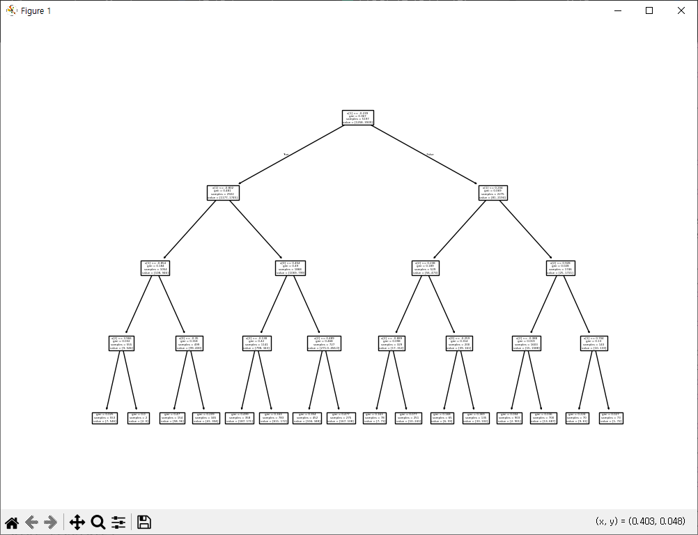
데이터를 지식으로 바꾸는 지능적인시스템구축
현대 기술 시대에는 정형 또는 비정형 데이터가 매우 풍부함
20세기 후반에 데이터에서 지식을 추출하여 예측하는 자기 학습(SELFLEARNING) 알고리즘과 관련된 인공 지능(ARTIFICIAL INTELLIGENCE, AI)의 하위 분야로 머신 러닝이 출현
사람이 수동으로 대량의 데이터를 분석하여 규칙을 유도하고 모델을 만듦
머신 러닝이 데이터에서 더 효율적으로 지식을 추출하여 예측 모델과 데이터 기반의 의사 결정 성능을 점진적으로 향상시킬 수 있음
컴퓨터 과학 연구에서 머신 러닝은 점점 더 중요해지며, 우리 일상생활에서도 아주 큰 역할을 하고 있음
머신 러닝 덕택에 견고한 이메일 스팸 필터, 편리한 텍스트와 음성 인식 소프트웨어, 믿을 수 있는 웹 검색 엔진, 체스 대결 프로그램을 사용
아마도 곧 안전하고 효율적인 자율 주행 자동차도 사용할 수 있을 것
또한 의료 애플리케이션에서도 큰 진전이 있었음
예를 들어 연구자들은 딥러닝 모델을 사용하여 피부암을 거의 사람 수준의 정확도로 진단 할 수 있다는 것을 보였음
최근에는 딥마인드(DEEPMIND)의 연구원들이 또 하나의 이정표를 세웠음
딥러닝으로 3D 단백질 구조를 예측하여 처음으로 물리학 기반 방식의 성능을 뛰어 넘었음
머신 러닝의 세 가지 종류
머신 러닝의 세 가지 종류는 지도학습(SUPERVISED LEARNING), 비지도 학습(UNSUPERVISED LEARNING), 강화 학습(REINFORCEMENT LEARNING) 입니다.
지도 학습 : 레이블된 데이터 , 직접 피드백, 출력 및 미래 예측
비지도 학습 : 레이블 및 타깃 없음, 피드백 없음, 데이터에서 숨겨진 구조 찾기
강화 학습 : 결정 과정, 보상 시스템, 연속된 행동에서 학습
지도 학습으로 미래 예측
지도 학습의 주요 목적은 레이블(LABEL)된 훈련 데이터에서 모델을 학습하여 본 적 없는 미래 데이터에 대해 예측을 만드는 것
여기서 지도(SUPERVISED) 는 희망하는 출력 신호 (레이블) 가 있는 일련의 샘플(데이터 입력)을 의미
레이블된 훈련 데이터가 머신 러닝 알고리즘에 전달되어 예측 모델을 훈련하고 그다음 새로운 레이블되지 않은 데이터 입력에 대해 예측을 수행
스팸 메일을 필터링하는 예를 생각해보면 레이블된 이메일 데이터셋에서 지도 학습 머신 러닝 알고리즘을 사용하여 모델을 훈련할 수 있음
이 데이터셋은 스팸 또는 스팸이 아닌 이메일로 정확하게 표시되어 있음
훈련된 모델은 새로운 이메일이 두 개의 범주(CATEGORY) 중 어디에 속하는지 예측
이메일 스팸 필터의 예처럼 개별 클래스 레이블이 있는 지도 학습을 분류(CLASSIFICATION) 라고 함
지도 학습의 또 다른 종류는 연속적인 값을 출력하는 회귀(REGRESSION)
분류 : 클래스 레이블 예측
분류는 지도 학습의 하위 카테고리
과거의 관측을 기반으로 새로운 샘플의 범주형 클래스 레이블을 예측 하는 것이 목적
클래스 레이블은 이산적(DISCRETE) 이고 순서가 없어 샘플이 속한 그룹으로 이해할 수 있음
앞서 언급한 스팸 메일 감지는 전형적인 이진 분류(BINARY CLASSIFICATION) 작업의 예
스팸과 스팸이 아닌 이메일 두 개의 클래스 사이를 구분하려고 머신 러닝 알고리즘이 일련의 규칙을 학습
두 개 이상의 클래스 레이블을 가진 경우가 많음
지도 학습 알고리즘으로 학습한 예측 모델은 훈련 데이터셋에 있는 클래스 레이블을 새로운 샘플에 할당할 수 있음
이런 다중 분류(MULTICLASS CLASSIFICATION) 의 전형적인 예는 손으로 쓴 글자 인식
여기서 글자("A","B","C" 등)는 예측하려는 대상이며 순서가 없는 범주나 클래스 레이블로 표현
알파벳 각 글자를 손으로 쓴 이미지 샘플을 모아서 훈련 데이터셋을 구성
새로운 글자를 입력으로 제공하면 예측 모델이 일정한 정확도로 알파벳 글자를 예측할 것
0에서 9까지 숫자가 훈련 데이터셋에 없다면 이 머신 러닝 시스템은 숫자를 인식하지 못할 것
회귀 : 연속적인 출력 값 예측
이전 절에서 분류 작업은 범주형 순서가 없는 레이블을 샘플에 할당하는 것이라고 배웟음
두 번째 지도 학습의 종류는 연속적인 출력 값을 예측하는 회귀 분석
회귀는 예측변수(PREDICTOR VARIABLE)(또는 설명 변수(EXPLANATORY VARIABLE) 와 연속적인 반응변수(RESPONSE VARIABLE)(또는 결과(OUTCOME))가 주어졌을 때 출력 값을 예측하기 위해 두 변수 사이의 관계를 찾음
중앙값
import numpy as np
import pandas as pd
import matplotlib.pyplot as plt

df = pd.read_csv('ch2_scores_em.csv', index_col='student number')
df.info()
print(df.head())
print()

scores = np.array(df['english'])[:10]
print(scores)

scores_df = pd.DataFrame({'score':scores},
                         index=pd.Index(list('ABCDEFGHIJ'), name='student'))
print(scores_df)
print()

sorted_scores = np.sort(scores)
print(sorted_scores)
print()

n = len(sorted_scores)
if n % 2 == 0:
    m0 = sorted_scores[n // 2 - 1]
    m1 = sorted_scores[n // 2]
    median = (m0 + m1) / 2
else:
    median = sorted_scores[(n+1)//2 - 1]

print(median)
print(np.median(scores))
print(scores_df.median())
print()

mean = np.mean(scores)
deviation = scores = mean
print(deviation)

another_scores = [50,60,58,54,51,56,57,53,67,59]
another_mean = np.mean(another_scores)
print(another_mean)
another_deviation = another_scores - another_mean
print(another_deviation)

print(np.mean(deviation))

summary_df = scores_df.copy()
summary_df['deviation'] = deviation
print(summary_df)
print()
print(np.mean(deviation ** 2))
print(np.var(scores))
print(scores_df.var(ddof=0))
print()

print(np.sqrt(np.mean(deviation ** 2)))
print()

z = (scores - np.mean(scores)) / np.std(scores)
print(z)

print(np.mean(z), round(np.std(z),3))
<class 'pandas.core.frame.DataFrame'>
Index: 50 entries, 1 to 50
Data columns (total 2 columns):
 #   Column       Non-Null Count  Dtype
---  ------       --------------  -----
 0   english      50 non-null     int64
 1   mathematics  50 non-null     int64
dtypes: int64(2)
memory usage: 1.2 KB
                english  mathematics
student number
1                    42           65
2                    69           80
3                    56           63
4                    41           63
5                    57           76

[42 69 56 41 57 48 65 49 65 58]
         score
student
A           42
B           69
C           56
D           41
E           57
F           48
G           65
H           49
I           65
J           58

[41 42 48 49 56 57 58 65 65 69]

56.5
56.5
score    56.5
dtype: float64

55.0
56.5
[-6.5  3.5  1.5 -2.5 -5.5 -0.5  0.5 -3.5 10.5  2.5]
55.0
         score  deviation
student
A           42       55.0
B           69       55.0
C           56       55.0
D           41       55.0
E           57       55.0
F           48       55.0
G           65       55.0
H           49       55.0
I           65       55.0
J           58       55.0

3025.0
0.0
score    86.0
dtype: float64

55.0

nan
nan nan
분산
import numpy as np
import pandas as pd
import matplotlib.pyplot as plt

df = pd.read_csv('ch2_scores_em.csv',index_col='student number')

en_scores = np.array(df['english'])[:10]
ma_scores = np.array(df['mathematics'])[:10]
scores_df = pd.DataFrame({'english':en_scores,
                          'mathematics': ma_scores},
                          index=pd.Index(list('ABCDEFGHIJ'),name='student'))
print(scores_df)

summary_df = scores_df.copy()
summary_df['english_deviation'] = summary_df['english'] - summary_df['english'].mean()
summary_df['mathematics_deviation'] = summary_df['mathematics'] - summary_df['mathematics'].mean()
summary_df['product_of_deviation'] = summary_df['english_deviation'] - summary_df['mathematics_deviation']

print(summary_df)
print()
print(summary_df['product_of_deviation'].mean())
print(np.cov(en_scores, ma_scores, ddof=0))
print()

print(round(np.cov(en_scores, ma_scores, ddof=0)[0,1]/(np.std(en_scores)*(np.std(ma_scores))),3))
print(np.corrcoef(en_scores, ma_scores))
print(scores_df.corr())

english_scores = np.array(df['english'])
math_scores = np.array(df['mathematics'])

fig = plt.figure(figsize=(7,7))
ax = fig.add_subplot(111)
ax.scatter(english_scores, math_scores)
ax.set_xlabel('english')
ax.set_ylabel('mathematics')
plt.show()

poly_fit = np.polyfit(english_scores, math_scores, deg=1)
print(poly_fit)
poly_1d = np.poly1d(poly_fit)
print(poly_1d)

xs = np.linspace(english_scores.min(), english_scores.max(), 50)
ys = poly_1d(xs)
fig = plt.figure(figsize=(7,7))
ax = fig.add_subplot(111)
ax.scatter(english_scores, math_scores, label='score')
ax.plot(xs,ys,color='gray',label=f'{poly_fit[0]:.2f}x + {poly_fit[1]:.2f}')
ax.legend(loc='best')
ax.set_xlabel('english')
ax.set_ylabel('mathematics')

plt.show()
         english  mathematics
student
A             42           65
B             69           80
C             56           63
D             41           63
E             57           76
F             48           60
G             65           81
H             49           66
I             65           78
J             58           82
         english  mathematics  ...  mathematics_deviation  product_of_deviation
student                        ...
A             42           65  ...                   -6.4                  -6.6
B             69           80  ...                    8.6                   5.4
C             56           63  ...                   -8.4                   9.4
D             41           63  ...                   -8.4                  -5.6
E             57           76  ...                    4.6                  -2.6
F             48           60  ...                  -11.4                   4.4
G             65           81  ...                    9.6                   0.4
H             49           66  ...                   -5.4                  -0.6
I             65           78  ...                    6.6                   3.4
J             58           82  ...                   10.6                  -7.6

[10 rows x 5 columns]

5.684341886080802e-15
[[86.   62.8 ]
 [62.8  68.44]]

0.819
[[1.         0.81856923]
 [0.81856923 1.        ]]
              english  mathematics
english      1.000000     0.818569
mathematics  0.818569     1.000000
[ 0.62142302 42.60132433]

0.6214 x + 42.6
머신러닝 세팅 모듈
머신러닝 샘플 만들기
from Tools.scripts.generate_token import make_c
from pandas.core.common import random_state
from sklearn.datasets import make_regression

features, target, coefficients = make_regression(n_samples=500,
                n_features=2,
                n_informative=2,
                n_targets=1,
                noise=0.0,
                coef=True,
                random_state=1)
# print(features)
# print(target)
print(features.shape)
print(target.shape)
print(coefficients)

import matplotlib.pyplot as plt
# plt.scatter(features[:,0], features[:,1], s=50, edgecolors='k')
# plt.show()

from sklearn.datasets import make_classification

features, targets = make_classification(n_samples=300,
                                        n_features=3,
                                        n_informative=3,
                                        n_redundant=0,
                                        n_classes=2,
                                        weights=[0.25,0.75],
                                        random_state=1)
print(features.shape)
print(targets)
(500, 2)
(500,)
[38.69892343 49.28808734]
(300, 3)
[1 0 1 1 1 0 1 1 1 1 0 1 0 1 1 1 1 0 0 1 1 0 1 1 0 1 1 1 0 1 1 0 0 0 0 1 1
 1 1 1 0 1 1 1 1 1 1 1 1 1 0 1 1 1 1 1 0 0 1 1 1 1 1 1 1 1 0 1 1 1 0 1 1 0
 0 1 0 1 1 0 1 0 1 1 1 1 0 1 1 1 0 1 1 1 0 0 1 1 1 1 1 1 1 1 1 0 1 1 0 1 1
 1 1 1 1 1 1 1 1 0 0 1 1 1 1 1 0 0 1 1 1 1 1 0 1 1 0 1 1 0 1 0 0 1 0 1 1 0
 1 1 1 1 1 0 0 1 1 0 1 1 1 1 1 1 0 0 1 1 1 1 1 1 0 1 1 1 1 1 1 1 1 1 1 1 1
 1 1 1 0 1 1 1 0 1 1 1 1 1 0 0 1 1 0 1 1 1 1 1 1 1 1 1 1 1 0 1 0 1 1 1 1 1
 1 1 1 1 0 1 1 1 0 0 1 1 1 1 0 0 0 1 1 1 0 0 1 1 1 1 0 1 1 1 1 1 0 1 1 1 1
 1 1 1 0 0 1 1 1 1 1 0 1 1 0 0 1 1 1 1 1 0 1 1 1 1 1 1 0 1 0 0 1 0 1 0 0 1
 1 1 1 1]
sklearn make_blobs
from sklearn.datasets import make_blobs

features, targets = make_blobs(n_samples=500,
                               n_features=2,
                               centers=4,
                               cluster_std=1,
                               shuffle=True,
                               random_state=1)

print(targets)
plt.scatter(features[:,0], features[:,-1], c=targets, s=100)
plt.show()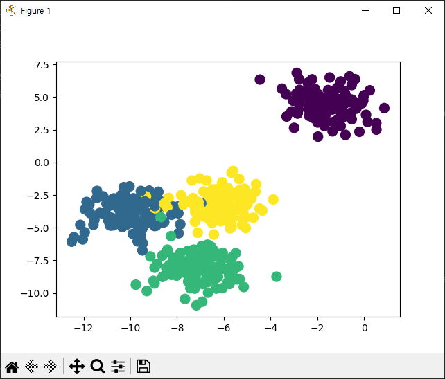
sklearn make_circles
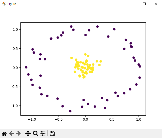
from sklearn.datasets import make_circles

features, targets = make_circles(n_samples=100,
                                 factor=0.1,
                                 noise=0.1)
plt.scatter(features[:,0], features[:,-1], c=targets)
plt.show()
sklearn make_moons
from sklearn.datasets import make_moons

features, targets = make_moons(n_samples = 400,
                               noise= 0.1,
                               random_state=1)
plt.scatter(features[:,0], features[:,-1], c=targets, marker='o', s=100)
plt.show()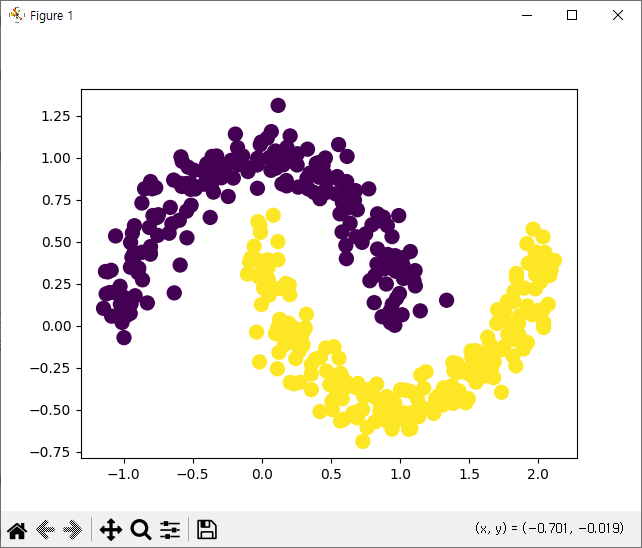
sklearn make_regression
from symbol import factor

from Tools.scripts.generate_token import make_c
from pandas.core.common import random_state
from sklearn.datasets import make_regression

features, target, coefficients = make_regression(n_samples=500,
                n_features=2,
                n_informative=2,
                n_targets=1,
                noise=0.0,
                coef=True,
                random_state=1)
# print(features)
# print(target)
print(features.shape)
print(target.shape)
print(coefficients)

import matplotlib.pyplot as plt
# plt.scatter(features[:,0], features[:,1], s=50, edgecolors='k')
# plt.show()

from sklearn.datasets import make_classification

features, targets = make_classification(n_samples=300,
                                        n_features=3,
                                        n_informative=3,
                                        n_redundant=0,
                                        n_classes=2,
                                        weights=[0.25,0.75],
                                        random_state=1)
print(features.shape)
print(targets)

from sklearn.datasets import make_blobs

features, targets = make_blobs(n_samples=500,
                               n_features=2,
                               centers=4,
                               cluster_std=1,
                               shuffle=True,
                               random_state=1)

print(targets)
# plt.scatter(features[:,0], features[:,-1], c=targets, s=100)
# plt.show()

from sklearn.datasets import make_circles

features, targets = make_circles(n_samples=100,
                                 factor=0.1,
                                 noise=0.1)
# plt.scatter(features[:,0], features[:,-1], c=targets)
# plt.show()

from sklearn.datasets import make_moons

features, targets = make_moons(n_samples = 400,
                               noise= 0.1,
                               random_state=1)
plt.scatter(features[:,0], features[:,-1], c=targets, marker='o', s=100)
plt.show()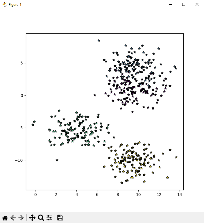
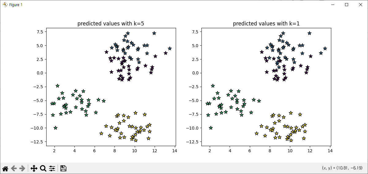
K-최근접 (KNN) train_test_split
from sklearn.model_selection import train_test_split
x_train, x_test, y_train, y_test = train_test_split(x,y, random_state=0)


knn5 = KNeighborsClassifier(n_neighbors=5)
knn1 = KNeighborsClassifier(n_neighbors=1)

knn5.fit(x_train,y_train)
knn1.fit(x_train,y_train)

y_pred5 = knn5.predict(x_test)
y_pred1 = knn1.predict(x_test)

from sklearn.metrics import accuracy_score

print('accuracy with k=5', accuracy_score(y_test, y_pred5 * 100))
print('accuracy with k=1', accuracy_score(y_test, y_pred1 * 100))

plt.figure(figsize=(12,5))
plt.subplot(121)
plt.scatter(x_test[:,0],x_test[:,1],c=y_pred5,marker='*',edgecolors='k',s=80)
plt.title('predicted values with k=5')

plt.subplot(122)
plt.scatter(x_test[:,0],x_test[:,1],c=y_pred1,marker='*',edgecolors='k',s=80)
plt.title('predicted values with k=1')

plt.show()
K-최근접 (KNN) KNeighborsClassifier
import matplotlib.pyplot as plt

bream_length = [25.4, 26.3, 26.5, 29.0, 29.0, 29.7, 29.7, 30.0, 30.0, 30.7, 31.0, 31.0, 31.5, 32.0, 32.0, 32.0, 33.0, 33.0, 33.5, 33.5, 34.0, 34.0, 34.5, 35.0, 35.0, 35.0, 35.0, 36.0, 36.0, 37.0, 38.5, 38.5, 39.5, 41.0, 41.0]
bream_weight = [242.0, 290.0, 340.0, 363.0, 430.0, 450.0, 500.0, 390.0, 450.0, 500.0, 475.0, 500.0, 500.0, 340.0, 600.0, 600.0, 700.0, 700.0, 610.0, 650.0, 575.0, 685.0, 620.0, 680.0, 700.0, 725.0, 720.0, 714.0, 850.0, 1000.0, 920.0, 955.0, 925.0, 975.0, 950.0]


smelt_length = [9.8, 10.5, 10.6, 11.0, 11.2, 11.3, 11.8, 11.8, 12.0, 12.2, 12.4, 13.0, 14.3, 15.0]
smelt_weight = [6.7, 7.5, 7.0, 9.7, 9.8, 8.7, 10.0, 9.9, 9.8, 12.2, 13.4, 12.2, 19.7, 19.9]

# plt.scatter(bream_length, bream_weight)
# plt.scatter(smelt_length, smelt_weight)
# plt.xlabel('length')
# plt.ylabel('weight')
# plt.show()

length = bream_length + smelt_length
weight = bream_weight + smelt_weight

fish_data = [[l,w] for l, w in zip(length,weight)]
print(fish_data)

fish_target = [1] * 35 + [0] * 14
print(fish_target)

from sklearn.neighbors import KNeighborsClassifier

kn = KNeighborsClassifier()
kn.fit(fish_data,fish_target)

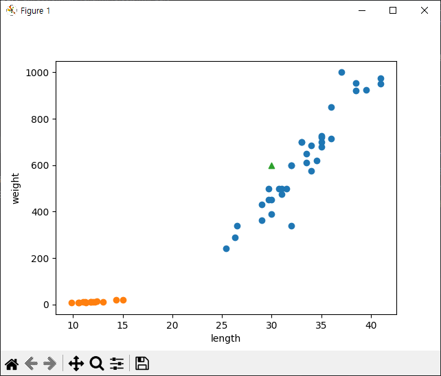
plt.scatter(bream_length, bream_weight)
plt.scatter(smelt_length, smelt_weight)
plt.scatter(30,600, marker='^')
plt.xlabel('length')
plt.ylabel('weight')
plt.show()

print()
print('length:30, weight:600 predict =>',kn.predict([[30,600]]))
print('accuracy:',kn.score(fish_data, fish_target))
[[25.4, 242.0], [26.3, 290.0], [26.5, 340.0], [29.0, 363.0], [29.0, 430.0], [29.7, 450.0], [29.7, 500.0], [30.0, 390.0], [30.0, 450.0], [30.7, 500.0], [31.0, 475.0], [31.0, 500.0], [31.5, 500.0], [32.0, 340.0], [32.0, 600.0], [32.0, 600.0], [33.0, 700.0], [33.0, 700.0], [33.5, 610.0], [33.5, 650.0], [34.0, 575.0], [34.0, 685.0], [34.5, 620.0], [35.0, 680.0], [35.0, 700.0], [35.0, 725.0], [35.0, 720.0], [36.0, 714.0], [36.0, 850.0], [37.0, 1000.0], [38.5, 920.0], [38.5, 955.0], [39.5, 925.0], [41.0, 975.0], [41.0, 950.0], [9.8, 6.7], [10.5, 7.5], [10.6, 7.0], [11.0, 9.7], [11.2, 9.8], [11.3, 8.7], [11.8, 10.0], [11.8, 9.9], [12.0, 9.8], [12.2, 12.2], [12.4, 13.4], [13.0, 12.2], [14.3, 19.7], [15.0, 19.9]]
[1, 1, 1, 1, 1, 1, 1, 1, 1, 1, 1, 1, 1, 1, 1, 1, 1, 1, 1, 1, 1, 1, 1, 1, 1, 1, 1, 1, 1, 1, 1, 1, 1, 1, 1, 0, 0, 0, 0, 0, 0, 0, 0, 0, 0, 0, 0, 0, 0]

length:30, weight:600 predict => [1]
accuracy: 1.0
sklearn KNeighborsRegressor
import numpy as np
import matplotlib.pyplot as plt


perch_length = np.array(
    [8.4, 13.7, 15.0, 16.2, 17.4, 18.0, 18.7, 19.0, 19.6, 20.0,
     21.0, 21.0, 21.0, 21.3, 22.0, 22.0, 22.0, 22.0, 22.0, 22.5,
     22.5, 22.7, 23.0, 23.5, 24.0, 24.0, 24.6, 25.0, 25.6, 26.5,
     27.3, 27.5, 27.5, 27.5, 28.0, 28.7, 30.0, 32.8, 34.5, 35.0,
     36.5, 36.0, 37.0, 37.0, 39.0, 39.0, 39.0, 40.0, 40.0, 40.0,
     40.0, 42.0, 43.0, 43.0, 43.5, 44.0]
     )
perch_weight = np.array(
    [5.9, 32.0, 40.0, 51.5, 70.0, 100.0, 78.0, 80.0, 85.0, 85.0,
     110.0, 115.0, 125.0, 130.0, 120.0, 120.0, 130.0, 135.0, 110.0,
     130.0, 150.0, 145.0, 150.0, 170.0, 225.0, 145.0, 188.0, 180.0,
     197.0, 218.0, 300.0, 260.0, 265.0, 250.0, 250.0, 300.0, 320.0,
     514.0, 556.0, 840.0, 685.0, 700.0, 700.0, 690.0, 900.0, 650.0,
     820.0, 850.0, 900.0, 1015.0, 820.0, 1100.0, 1000.0, 1100.0,
     1000.0, 1000.0]
     )

# plt.scatter(perch_length, perch_weight)
# plt.xlabel('length')
# plt.ylabel('weight')
# plt.show()

from sklearn.model_selection import train_test_split

x_train, x_test, y_train, y_test = train_test_split(
    perch_length, perch_weight, random_state=42
)

print(x_train.shape, x_test.shape)

x_train = x_train.reshape(-1,1)
x_test = x_test.reshape(-1, 1)
print(x_train.shape)
print(x_train)

from sklearn.neighbors import KNeighborsRegressor

knr = KNeighborsRegressor()
knr.fit(x_train, y_train)
print('accuracy:', knr.score(x_test,y_test))
print()

knr2 = KNeighborsRegressor(n_neighbors=3)
knr2.fit(x_train, y_train)
print('n_neighbors=3, accuracy :', knr2.score(x_test, y_test))
print()

knr = KNeighborsRegressor()
x = np.arange(5, 45).reshape(-1,1)

plt.figure(figsize=(4,12))
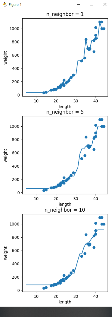
for idx,n in enumerate([1,5,10]):
    knr.n_neighbors = n
    knr.fit(x_train, y_train)
    prediction = knr.predict(x)
    plt.subplot(3,1,idx+1)
    plt.scatter(x_train, y_train)
    plt.plot(x, prediction)
    plt.xlabel('length')
    plt.ylabel('weight')
    plt.title(f'n_neighbor = {n}')

plt.tight_layout()
plt.show()
sklearn LinearRegression
import numpy as np
import matplotlib.pyplot as plt


perch_length = np.array(
    [8.4, 13.7, 15.0, 16.2, 17.4, 18.0, 18.7, 19.0, 19.6, 20.0,
     21.0, 21.0, 21.0, 21.3, 22.0, 22.0, 22.0, 22.0, 22.0, 22.5,
     22.5, 22.7, 23.0, 23.5, 24.0, 24.0, 24.6, 25.0, 25.6, 26.5,
     27.3, 27.5, 27.5, 27.5, 28.0, 28.7, 30.0, 32.8, 34.5, 35.0,
     36.5, 36.0, 37.0, 37.0, 39.0, 39.0, 39.0, 40.0, 40.0, 40.0,
     40.0, 42.0, 43.0, 43.0, 43.5, 44.0]
     )
perch_weight = np.array(
    [5.9, 32.0, 40.0, 51.5, 70.0, 100.0, 78.0, 80.0, 85.0, 85.0,
     110.0, 115.0, 125.0, 130.0, 120.0, 120.0, 130.0, 135.0, 110.0,
     130.0, 150.0, 145.0, 150.0, 170.0, 225.0, 145.0, 188.0, 180.0,
     197.0, 218.0, 300.0, 260.0, 265.0, 250.0, 250.0, 300.0, 320.0,
     514.0, 556.0, 840.0, 685.0, 700.0, 700.0, 690.0, 900.0, 650.0,
     820.0, 850.0, 900.0, 1015.0, 820.0, 1100.0, 1000.0, 1100.0,
     1000.0, 1000.0]
     )

from sklearn.model_selection import train_test_split

x_train, x_test, y_train, y_test = train_test_split(
    perch_length, perch_weight, random_state=42
)

x_train = x_train.reshape(-1,1)
x_test = x_test.reshape(-1, 1)

from sklearn.neighbors import KNeighborsRegressor

knr = KNeighborsRegressor()
knr.fit(x_train, y_train)
print(knr.predict([[50]]))
print()

# distances, indexes = knr.kneighbors([[50]])
# print(distances, indexes)
#
# plt.scatter(x_train, y_train)
# plt.scatter(x_train[indexes], y_train[indexes], marker='D')
# plt.scatter(100,1033,marker='^')
# plt.show()

from sklearn.linear_model import LinearRegression

lr = LinearRegression()
lr.fit(x_train, y_train)
print(lr.predict([[50]]))
print(lr.coef_,lr.intercept_)

# plt.scatter(x_train, y_train)
# plt.plot([15,50], [15*lr.coef_ +lr.intercept_, 50*lr.coef_ + lr.intercept_])
# plt.scatter(50,1241,marker='^')
# plt.show()

train_poly = np.column_stack((x_train ** 2, x_train))
test_poly = np.column_stack((x_test ** 2, x_test))
print(train_poly)

lr= LinearRegression()
lr.fit(train_poly, y_train)

print(lr.predict([[50**2, 50]]))
print(lr.coef_, lr.intercept_)

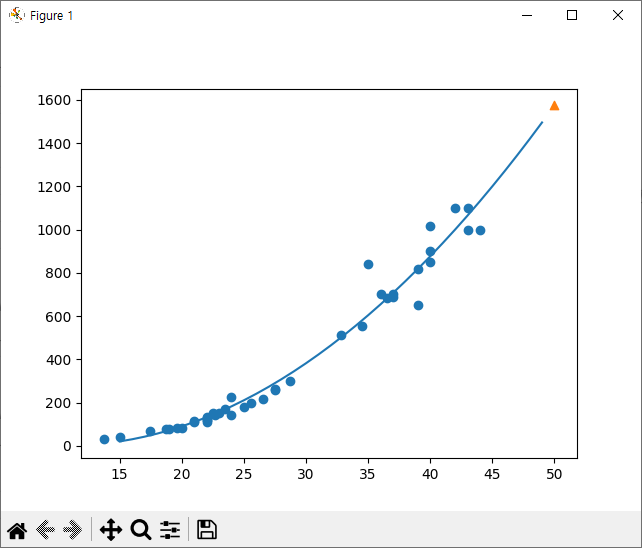
point = np.arange(15, 50)
plt.scatter(x_train, y_train)
plt.plot(point, 1.01433211*point**2 -21.55792498*point + 116.0502107827827)
plt.scatter(50,1574, marker='^')
plt.show()
logisticModel , StandardScaler
import matplotlib.pyplot as plt
import pandas as pd

from day2.KNNEx3 import fish_target

fish = pd.read_csv('https://bit.ly/fish_csv')
fish.info()
print(fish.head(10))
print(fish.Species.unique())

fish_input = fish.iloc[:,1:].values
# print(fish_input)
print(fish_input.shape)

fish_target = fish['Species'].to_numpy()
print(fish_target)

from sklearn.model_selection import train_test_split

train_input, test_input, train_target, test_target = train_test_split(
    fish_input, fish_target, random_state=42
)

from sklearn.preprocessing import StandardScaler

ss = StandardScaler()
ss.fit(train_input)
train_scaled = ss.transform(train_input)
print(train_scaled[1])
test_scaled = ss.transform(test_input)

from sklearn.neighbors import KNeighborsClassifier

kn = KNeighborsClassifier(n_neighbors=3)
kn.fit(train_scaled, train_target)
print('KNN model (train data) accuracy:',kn.score(train_scaled, train_target))
print('KNN model (test data) accuracy:',kn.score(test_scaled, test_target))
print(kn.classes_)

import numpy as np
proba = kn.predict_proba(test_scaled[:5])
print(np.round(proba, 4))

bream_smelt_indexes = (train_target == 'Bream')| (train_target == 'Smelt')
train_bream_smelt = train_scaled[bream_smelt_indexes]
target_bream_smelt = train_target[bream_smelt_indexes]
print(train_bream_smelt)
print(target_bream_smelt)

from sklearn.linear_model import LogisticRegression

lr = LogisticRegression()
lr.fit(train_bream_smelt, target_bream_smelt)
print()
print(lr.predict(train_bream_smelt[:5]))
print()
print(lr.predict_proba(train_bream_smelt[:5]))

lr = LogisticRegression(C=30,max_iter=1000)
lr.fit(train_scaled, train_target)
print(lr.score(train_scaled, train_target))
[[1 4 7]
 [2 5 8]
 [3 6 9]]
[[  25.4  242. ]
 [  26.3  290. ]
 [  26.5  340. ]
 [  29.   363. ]
 [  29.   430. ]
 [  29.7  450. ]
 [  29.7  500. ]
 [  30.   390. ]
 [  30.   450. ]
 [  30.7  500. ]
 [  31.   475. ]
 [  31.   500. ]
 [  31.5  500. ]
 [  32.   340. ]
 [  32.   600. ]
 [  32.   600. ]
 [  33.   700. ]
 [  33.   700. ]
 [  33.5  610. ]
 [  33.5  650. ]
 [  34.   575. ]
 [  34.   685. ]
 [  34.5  620. ]
 [  35.   680. ]
 [  35.   700. ]
 [  35.   725. ]
 [  35.   720. ]
 [  36.   714. ]
 [  36.   850. ]
 [  37.  1000. ]
 [  38.5  920. ]
 [  38.5  955. ]
 [  39.5  925. ]
 [  41.   975. ]
 [  41.   950. ]
 [   9.8    6.7]
 [  10.5    7.5]
 [  10.6    7. ]
 [  11.     9.7]
 [  11.2    9.8]
 [  11.3    8.7]
 [  11.8   10. ]
 [  11.8    9.9]
 [  12.     9.8]
 [  12.2   12.2]
 [  12.4   13.4]
 [  13.    12.2]
 [  14.3   19.7]
 [  15.    19.9]]
[1. 1. 1. 1. 1. 1. 1. 1. 1. 1. 1. 1. 1. 1. 1. 1. 1. 1. 1. 1. 1. 1. 1. 1.
 1. 1. 1. 1. 1. 1. 1. 1. 1. 1. 1. 0. 0. 0. 0. 0. 0. 0. 0. 0. 0. 0. 0. 0.
 0.]
(36, 2) (13, 2)

[[  30.   450. ]
 [  29.   363. ]
 [  29.7  500. ]
 [  11.3    8.7]
 [  11.8   10. ]
 [  13.    12.2]
 [  32.   600. ]
 [  30.7  500. ]
 [  33.   700. ]
 [  35.   700. ]
 [  41.   975. ]
 [  38.5  920. ]
 [  25.4  242. ]
 [  12.     9.8]
 [  39.5  925. ]
 [  29.7  450. ]
 [  37.  1000. ]
 [  31.   500. ]
 [  10.5    7.5]
 [  26.3  290. ]
 [  34.   685. ]
 [  26.5  340. ]
 [  10.6    7. ]
 [   9.8    6.7]
 [  35.   680. ]
 [  11.2    9.8]
 [  31.   475. ]
 [  34.5  620. ]
 [  33.5  610. ]
 [  15.    19.9]
 [  34.   575. ]
 [  30.   390. ]
 [  11.8    9.9]
 [  32.   600. ]
 [  36.   850. ]
 [  11.     9.7]]

test data accuracy: 1.0
[1. 0. 0. 0. 1. 1. 1. 1. 1. 1. 1. 1. 1.]
[1. 0. 0. 0. 1. 1. 1. 1. 1. 1. 1. 1. 1.]
<class 'pandas.core.frame.DataFrame'>
RangeIndex: 159 entries, 0 to 158
Data columns (total 6 columns):
 #   Column    Non-Null Count  Dtype
---  ------    --------------  -----
 0   Species   159 non-null    object
 1   Weight    159 non-null    float64
 2   Length    159 non-null    float64
 3   Diagonal  159 non-null    float64
 4   Height    159 non-null    float64
 5   Width     159 non-null    float64
dtypes: float64(5), object(1)
memory usage: 7.6+ KB
  Species  Weight  Length  Diagonal   Height   Width
0   Bream   242.0    25.4      30.0  11.5200  4.0200
1   Bream   290.0    26.3      31.2  12.4800  4.3056
2   Bream   340.0    26.5      31.1  12.3778  4.6961
3   Bream   363.0    29.0      33.5  12.7300  4.4555
4   Bream   430.0    29.0      34.0  12.4440  5.1340
5   Bream   450.0    29.7      34.7  13.6024  4.9274
6   Bream   500.0    29.7      34.5  14.1795  5.2785
7   Bream   390.0    30.0      35.0  12.6700  4.6900
8   Bream   450.0    30.0      35.1  14.0049  4.8438
9   Bream   500.0    30.7      36.2  14.2266  4.9594
['Bream' 'Roach' 'Whitefish' 'Parkki' 'Perch' 'Pike' 'Smelt']
(159, 5)
['Bream' 'Bream' 'Bream' 'Bream' 'Bream' 'Bream' 'Bream' 'Bream' 'Bream'
 'Bream' 'Bream' 'Bream' 'Bream' 'Bream' 'Bream' 'Bream' 'Bream' 'Bream'
 'Bream' 'Bream' 'Bream' 'Bream' 'Bream' 'Bream' 'Bream' 'Bream' 'Bream'
 'Bream' 'Bream' 'Bream' 'Bream' 'Bream' 'Bream' 'Bream' 'Bream' 'Roach'
 'Roach' 'Roach' 'Roach' 'Roach' 'Roach' 'Roach' 'Roach' 'Roach' 'Roach'
 'Roach' 'Roach' 'Roach' 'Roach' 'Roach' 'Roach' 'Roach' 'Roach' 'Roach'
 'Roach' 'Whitefish' 'Whitefish' 'Whitefish' 'Whitefish' 'Whitefish'
 'Whitefish' 'Parkki' 'Parkki' 'Parkki' 'Parkki' 'Parkki' 'Parkki'
 'Parkki' 'Parkki' 'Parkki' 'Parkki' 'Parkki' 'Perch' 'Perch' 'Perch'
 'Perch' 'Perch' 'Perch' 'Perch' 'Perch' 'Perch' 'Perch' 'Perch' 'Perch'
 'Perch' 'Perch' 'Perch' 'Perch' 'Perch' 'Perch' 'Perch' 'Perch' 'Perch'
 'Perch' 'Perch' 'Perch' 'Perch' 'Perch' 'Perch' 'Perch' 'Perch' 'Perch'
 'Perch' 'Perch' 'Perch' 'Perch' 'Perch' 'Perch' 'Perch' 'Perch' 'Perch'
 'Perch' 'Perch' 'Perch' 'Perch' 'Perch' 'Perch' 'Perch' 'Perch' 'Perch'
 'Perch' 'Perch' 'Perch' 'Perch' 'Perch' 'Perch' 'Perch' 'Perch' 'Pike'
 'Pike' 'Pike' 'Pike' 'Pike' 'Pike' 'Pike' 'Pike' 'Pike' 'Pike' 'Pike'
 'Pike' 'Pike' 'Pike' 'Pike' 'Pike' 'Pike' 'Smelt' 'Smelt' 'Smelt' 'Smelt'
 'Smelt' 'Smelt' 'Smelt' 'Smelt' 'Smelt' 'Smelt' 'Smelt' 'Smelt' 'Smelt'
 'Smelt']
[ 0.30041219  1.54653445  1.45316551 -0.46981663  0.27291745]
KNN model (train data) accuracy: 0.8907563025210085
KNN model (test data) accuracy: 0.85
['Bream' 'Parkki' 'Perch' 'Pike' 'Roach' 'Smelt' 'Whitefish']
[[0.     0.     1.     0.     0.     0.     0.    ]
 [0.     0.     0.     0.     0.     1.     0.    ]
 [0.     0.     0.     1.     0.     0.     0.    ]
 [0.     0.     0.6667 0.     0.3333 0.     0.    ]
 [0.     0.     0.6667 0.     0.3333 0.     0.    ]]
 [ 0.30041219  1.54653445  1.45316551 -0.46981663  0.27291745]
[[ 0.91965782  0.60943175  0.81041221  1.85194896  1.00075672]
 [-1.0858536  -1.68646987 -1.70848587 -1.70159849 -2.0044758 ]
 [ 0.63818253  0.56257661  0.73223951  1.64473401  0.50705737]
 [ 0.30041219  0.23459067  0.42823457  1.36042157  0.22329758]
 [ 0.9027693   0.70314202  0.88858491  1.89027545  0.85537174]
 [-1.0824759  -1.61150165 -1.62162731 -1.7000674  -1.92815631]
 [ 0.10337949  0.04717013  0.23714575  0.88445197  0.41799764]
 [ 1.49668216  1.03112796  1.21864741  2.44274986  1.40289707]
 [ 0.23004337  0.23459067  0.42823457  1.3336029   0.39983213]
 [-0.42579405 -0.29018684 -0.11028847  0.65627104 -0.26107519]
 [ 1.28557569  0.70314202  0.89727076  1.98228866  1.06683526]
 [ 0.93373158  0.60943175  0.83646978  1.85150445  0.97832415]
 [ 0.80706771  0.60943175  0.81041221  1.63137406  1.0255057 ]
 [-1.07262426 -1.52716241 -1.55214047 -1.67235972 -1.86207776]
 [ 1.6374198   1.17169337  1.27076255  2.41341232  1.40143407]
 [-1.07966115 -1.63961473 -1.67374245 -1.6462819  -1.87036806]
 [-1.05151362 -1.33037084 -1.39579507 -1.47914678 -1.45146425]
 [ 0.15967454  0.11276732  0.29794674  1.17051775  0.29205828]
 [ 1.56705098  1.17169337  1.32287768  2.16352457  1.17174409]
 [-0.00921063  0.1408804   0.3240043   0.94026245  0.14734384]
 [ 0.15967454  0.1408804   0.33269016  1.26991474  0.24109734]
 [-0.14994827  0.32830094  0.52377898  1.24719543  0.3806913 ]
 [-0.08520896  0.04717013  0.19371647  0.95507939  0.00439718]
 [ 0.86336276  0.42201121  0.62800925  1.5003429   0.45670601]
 [ 0.30041219  0.11276732  0.28057503  1.31303204  0.50608204]
 [-1.07262426 -1.45219419 -1.51739705 -1.62627903 -1.94607798]
 [ 0.82114147  0.51572148  0.68881023  1.76102232  0.5621025 ]
 [-1.07937967 -1.54590446 -1.56951218 -1.64420753 -2.01154694]
 [-1.07937967 -1.62087268 -1.63899902 -1.67413775 -1.93303295]
 [-0.29068592 -0.2058476  -0.0060582   0.89334213 -0.08697896]
 [-1.05095067 -1.26477365 -1.30893652 -1.46447801 -1.56606541]
 [ 0.51151865  0.51572148  0.7148678   1.54738669  0.68347   ]
 [ 0.58188748  0.32830094  0.51509312  1.50439286  0.4404302 ]]
['Bream' 'Smelt' 'Bream' 'Bream' 'Bream' 'Smelt' 'Bream' 'Bream' 'Bream'
 'Bream' 'Bream' 'Bream' 'Bream' 'Smelt' 'Bream' 'Smelt' 'Smelt' 'Bream'
 'Bream' 'Bream' 'Bream' 'Bream' 'Bream' 'Bream' 'Bream' 'Smelt' 'Bream'
 'Smelt' 'Smelt' 'Bream' 'Smelt' 'Bream' 'Bream']

['Bream' 'Smelt' 'Bream' 'Bream' 'Bream']

[[0.99760007 0.00239993]
 [0.02737325 0.97262675]
 [0.99486386 0.00513614]
 [0.98585047 0.01414953]
 [0.99767419 0.00232581]]

 0.9663865546218487
Deicison Tree 디시전 트리
import numpy as np
import matplotlib.pyplot as plt
from matplotlib.colors import ListedColormap


def plot_decision_boundary(clf, X, y, axes=[0, 7.5, 0, 3], iris=True, legend=False, plot_training=True):
    x1s = np.linspace(axes[0], axes[1], 100)
    x2s = np.linspace(axes[2], axes[3], 100)
    x1, x2 = np.meshgrid(x1s, x2s)
    X_new = np.c_[x1.ravel(), x2.ravel()]
    y_pred = clf.predict(X_new).reshape(x1.shape)
    custom_cmap = ListedColormap(['#fafab0','#9898ff','#a0faa0'])
    plt.contourf(x1, x2, y_pred, alpha=0.3, cmap=custom_cmap)
    if not iris:
        custom_cmap2 = ListedColormap(['#7d7d58','#4c4c7f','#507d50'])
        plt.contour(x1, x2, y_pred, cmap=custom_cmap2, alpha=0.8)
    if plot_training:
        plt.plot(X[:, 0][y==0], X[:, 1][y==0], "yo", label="Iris setosa")
        plt.plot(X[:, 0][y==1], X[:, 1][y==1], "bs", label="Iris versicolor")
        plt.plot(X[:, 0][y==2], X[:, 1][y==2], "g^", label="Iris virginica")
        plt.axis(axes)
    if iris:
        plt.xlabel("Petal length", fontsize=14)
        plt.ylabel("Petal width", fontsize=14)
    else:
        plt.xlabel(r"$x_1$", fontsize=18)
        plt.ylabel(r"$x_2$", fontsize=18, rotation=0)
    if legend:
        plt.legend(loc="lower right", fontsize=14)


from sklearn.datasets import load_iris

iris = load_iris()
print(iris.keys())
print(iris.DESCR)
print(iris.target)
print(iris.target_names)
print(iris.feature_names)

x = iris.data[:,2:]
y = iris.target

from sklearn.tree import DecisionTreeClassifier
tree_clf = DecisionTreeClassifier(max_depth=2, random_state=42)
tree_clf.fit(x,y)

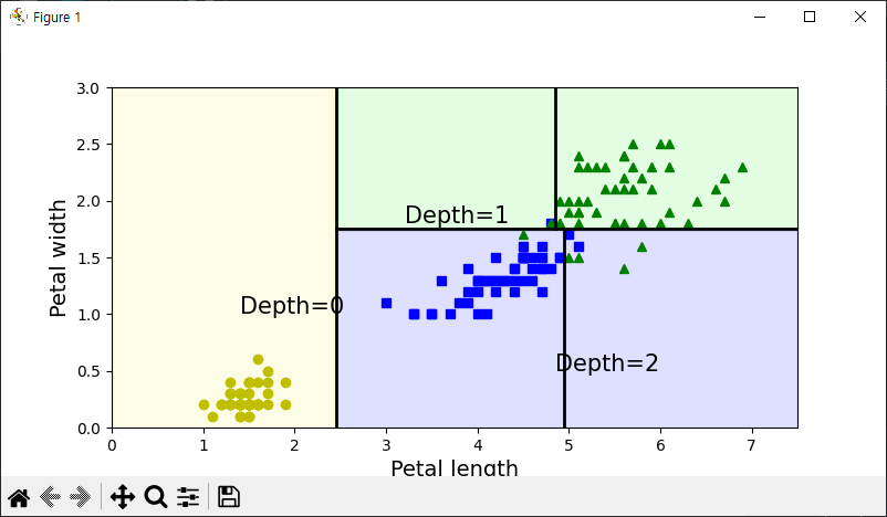
plt.figure(figsize=(8,4))
plot_decision_boundary(tree_clf,x,y)
plt.plot([2.45,2.45],[0,3],'k-',linewidth=2)
plt.plot([2.45,7.5],[1.75,1.75],'k-',linewidth=2)
plt.plot([4.95,4.95],[0,1.75],'k-',linewidth=2)
plt.plot([4.85,4.85],[1.75,3],'k-',linewidth=2)
plt.text(1.4,1,'Depth=0',fontsize=15)
plt.text(3.2,1.8,'Depth=1',fontsize=15)
plt.text(4.85,0.5,'Depth=2',fontsize=15)

plt.show()
추가
from sklearn.datasets import make_moons

xm, ym = make_moons(n_samples=100, noise=0.25, random_state=53)

dtree_clf1 = DecisionTreeClassifier(random_state=42)
dtree_clf2 = DecisionTreeClassifier(min_samples_leaf=4,random_state=42)

dtree_clf1.fit(xm,ym)
dtree_clf2.fit(xm,ym)

fig, axes = plt.subplots(ncols=2, figsize=(10,4))
plt.sca(axes[0])
plot_decision_boundary(dtree_clf1, xm, ym, axes=[-1.5,2.4,-1,1.5], iris = False)
plt.title('no restrictions', fontsize=16)

plt.sca(axes[1])
plot_decision_boundary(dtree_clf2, xm, ym, axes=[-1.5,2.4,-1,1.5], iris = False)
plt.title(f'min_samples_leaf={dtree_clf2.min_samples_leaf}', fontsize=16)
plt.ylabel('')
plt.show()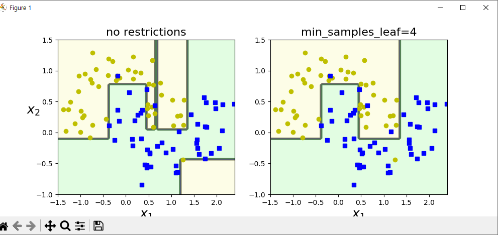
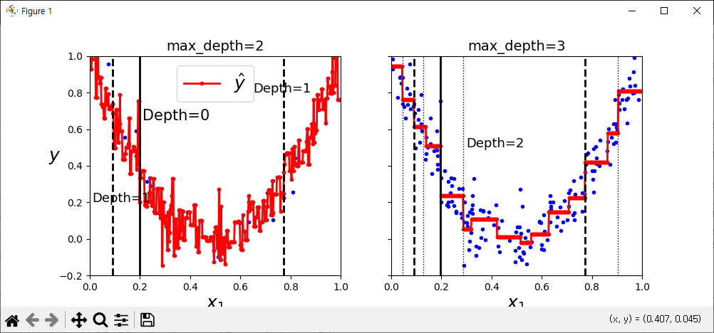
import numpy as np
import matplotlib.pyplot as plt
from sklearn.tree import DecisionTreeRegressor

np.random.seed(42)
m = 200
X = np.random.rand(m,1)
y = 4 * (X-0.5) ** 2
y = y + np.random.randn(m,1)/10

# tree_reg1 = DecisionTreeRegressor(random_state=42, max_depth=2)
# tree_reg2 = DecisionTreeRegressor(random_state=42, max_depth=3)

tree_reg1 = DecisionTreeRegressor(random_state=42)
tree_reg2 = DecisionTreeRegressor(random_state=42,min_samples_leaf=10)

tree_reg1.fit(X,y)
tree_reg2.fit(X,y)

def plot_regression_predictions(tree_reg, X, y, axes=[0, 1, -0.2, 1], ylabel="$y$"):
    x1 = np.linspace(axes[0], axes[1], 500).reshape(-1, 1)
    y_pred = tree_reg.predict(x1)
    plt.axis(axes)
    plt.xlabel("$x_1$", fontsize=18)
    if ylabel:
        plt.ylabel(ylabel, fontsize=18, rotation=0)
    plt.plot(X, y, "b.")
    plt.plot(x1, y_pred, "r.-", linewidth=2, label=r"$\hat{y}$")

fig, axes = plt.subplots(ncols=2, figsize=(10, 4), sharey=True)
plt.sca(axes[0])
plot_regression_predictions(tree_reg1, X, y)
for split, style in ((0.1973, "k-"), (0.0917, "k--"), (0.7718, "k--")):
    plt.plot([split, split], [-0.2, 1], style, linewidth=2)
plt.text(0.21, 0.65, "Depth=0", fontsize=15)
plt.text(0.01, 0.2, "Depth=1", fontsize=13)
plt.text(0.65, 0.8, "Depth=1", fontsize=13)
plt.legend(loc="upper center", fontsize=18)
plt.title("max_depth=2", fontsize=14)

plt.sca(axes[1])
plot_regression_predictions(tree_reg2, X, y, ylabel=None)
for split, style in ((0.1973, "k-"), (0.0917, "k--"), (0.7718, "k--")):
    plt.plot([split, split], [-0.2, 1], style, linewidth=2)
for split in (0.0458, 0.1298, 0.2873, 0.9040):
    plt.plot([split, split], [-0.2, 1], "k:", linewidth=1)
plt.text(0.3, 0.5, "Depth=2", fontsize=13)
plt.title("max_depth=3", fontsize=14)

plt.show()


# fig, axes = plt.subplots(ncols=2, figsize=(10, 4), sharey=True)
#
# plt.sca(axes[0])
# plt.plot(X, y, "b.")
# plt.plot(x1, y_pred1, "r.-", linewidth=2, label=r"$\hat{y}$")
# plt.axis([0, 1, -0.2, 1.1])
# plt.xlabel("$x_1$", fontsize=18)
# plt.ylabel("$y$", fontsize=18, rotation=0)
# plt.legend(loc="upper center", fontsize=18)
# plt.title("No restrictions", fontsize=14)
#
# plt.sca(axes[1])
# plt.plot(X, y, "b.")
# plt.plot(x1, y_pred2, "r.-", linewidth=2, label=r"$\hat{y}$")
# plt.axis([0, 1, -0.2, 1.1])
# plt.xlabel("$x_1$", fontsize=18)
# plt.title("min_samples_leaf={}".format(tree_reg2.min_samples_leaf), fontsize=14)
# plt.show()
import pandas as pd

wine = pd.read_csv('https://bit.ly/wine-date')
wine.info()
print(wine.head(15))
print(wine['class'].unique())

data = wine[['alcohol', 'sugar', 'pH']].to_numpy()
target = wine['class'].to_numpy()
print(data)
print(target)

from sklearn.model_selection import train_test_split

x_train, x_test, y_train, y_test = train_test_split(
    data, target, test_size=0.2, random_state=42
)

print(x_train.shape, x_test.shape)

from sklearn.preprocessing import StandardScaler

ss = StandardScaler()
ss.fit(x_train)

x_train_scaled = ss.transform(x_train)
x_test_scaled = ss.transform(x_test)
print(x_train_scaled)

from sklearn.linear_model import LogisticRegression

lr = LogisticRegression()
lr.fit(x_train_scaled, y_train)
print(lr.score(x_train_scaled, y_train))
print(lr.score(x_test_scaled, y_test))

from sklearn.tree import DecisionTreeClassifier
dt = DecisionTreeClassifier(random_state=42)
dt.fit(x_train_scaled, y_train)
print(dt.score(x_train_scaled, y_train))
print(dt.score(x_test_scaled, y_test))

dt2 = DecisionTreeClassifier(max_depth=4, random_state=42)
dt2.fit(x_train_scaled, y_train)
print(dt2.score(x_train_scaled, y_train))
print(dt2.score(x_test_scaled, y_test))

import matplotlib.pyplot as plt
from sklearn.tree import plot_tree
plt.figure(figsize=(10,7))
plot_tree(dt2)
plt.show()