머신러닝( SVM , 커널, 앙상블)

짬그브·2025년 3월 19일

커널 서포트 벡터 머신

서포트 벡터 머신 (Support Vector Machine : SVM)은 각 훈련 데이터 포인트 들의 클래스 결정 경계를 구분하는 것을 학습한다.
일반적으로 훈련 데이터의 일부, 두 클래스 사이의 경계에 위치한 데이터 포인트들만 결정 경계를 만드는데 영향을 준다. 이런 데이터 포인트를 서포트벡터(Support Vector) 라 하며, 여기서 서포트 벡터 머신이라는 이름이 유래 되었다.
새로운 데이터 포인트에 대해 예측할 때는, 데이터 포인트와 각 서포트 벡터와의 거리를 측정한다. 즉 서포터 벡터 머신은 서로 다른 클래스를 지닌 데이터 사이의 간격이 최대가 되는 선이나 평면을 찾아 이를 기준으로 각 데이터들을 분류하는 모델이다. 다시 말해 데이터 사이에 존재하는 여백을 최대화, 일반화하여 성능을 극대화한 모델이다.

Kernel-SVM 의 핵심 아이디어는 원공간(Input Space)의 데이터를 선형 분류가 가능한 고차원 공간(Feature Space)으로 매핑한 뒤 두 범주를 분류하는 초 평면을 찾는 것이다.
복잡한 형태의 데이터 셋에 비선형 특성을 추가하면 선형모델을 강력하게 만들 수 있지만 연산 비용이 커지는 문제가 발생한다
고차원 매핑과 내적을 한번에 하기 위해 도입된 것이 커널 이다.

대표적인 커널

선형 서포트 벡터 머신

다항 커널(Polynomial Kernel)

RBF(Radial Basis Function) 또는 가우시안 커널(Gaussian Kernel)

시그모이드 커널(Sigmoid Kernel)

import matplotlib.pyplot as plt
import numpy as np
from sklearn.datasets import make_moons

X, y = make_moons(n_samples=100, noise=0.15, random_state=42)


X1D = np.linspace(-4, 4, 9).reshape(-1, 1)
X2D = np.c_[X1D, X1D**2]

def gaussian_rbf(x, landmark, gamma):
    return np.exp(-gamma * np.linalg.norm(x - landmark, axis=1)**2)

gamma = 0.3

x1s = np.linspace(-4.5, 4.5, 200).reshape(-1, 1)
x2s = gaussian_rbf(x1s, -2, gamma)
x3s = gaussian_rbf(x1s, 1, gamma)

XK = np.c_[gaussian_rbf(X1D, -2, gamma), gaussian_rbf(X1D, 1, gamma)]
yk = np.array([0, 0, 1, 1, 1, 1, 1, 0, 0])

plt.figure(figsize=(10.5, 4))

plt.subplot(121)
plt.grid(True, which='both')
plt.axhline(y=0, color='k')
plt.scatter(x=[-2, 1], y=[0, 0], s=150, alpha=0.5, c="red")
plt.plot(X1D[:, 0][yk==0], np.zeros(4), "bs")
plt.plot(X1D[:, 0][yk==1], np.zeros(5), "g^")
plt.plot(x1s, x2s, "g--")
plt.plot(x1s, x3s, "b:")
plt.gca().get_yaxis().set_ticks([0, 0.25, 0.5, 0.75, 1])
plt.xlabel(r"$x_1$", fontsize=20)
plt.ylabel(r"Similarity", fontsize=14)
plt.annotate(r'$\mathbf{x}$',
             xy=(X1D[3, 0], 0),
             xytext=(-0.5, 0.20),
             ha="center",
             arrowprops=dict(facecolor='black', shrink=0.1),
             fontsize=18,
            )
plt.text(-2, 0.9, "$x_2$", ha="center", fontsize=20)
plt.text(1, 0.9, "$x_3$", ha="center", fontsize=20)
plt.axis([-4.5, 4.5, -0.1, 1.1])

plt.subplot(122)
plt.grid(True, which='both')
plt.axhline(y=0, color='k')
plt.axvline(x=0, color='k')
plt.plot(XK[:, 0][yk==0], XK[:, 1][yk==0], "bs")
plt.plot(XK[:, 0][yk==1], XK[:, 1][yk==1], "g^")
plt.xlabel(r"$x_2$", fontsize=20)
plt.ylabel(r"$x_3$", fontsize=20, rotation=0)
plt.annotate(r'$\phi\left(\mathbf{x}\right)$',
             xy=(XK[3, 0], XK[3, 1]),
             xytext=(0.65, 0.50),
             ha="center",
             arrowprops=dict(facecolor='black', shrink=0.1),
             fontsize=18,
            )
plt.plot([-0.1, 1.1], [0.57, -0.1], "r--", linewidth=3)
plt.axis([-0.1, 1.1, -0.1, 1.1])

plt.subplots_adjust(right=1)

plt.show()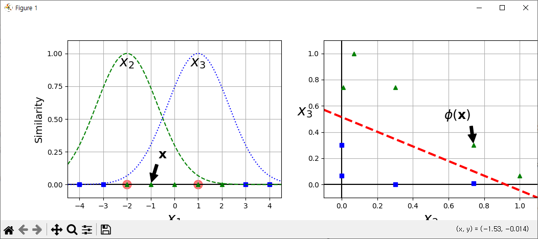

감마(Γ) 값이 증가하면 종모양 좁아지고 샘플에 해당하는 영향력이 약해짐
감마(Γ) 값이 낮아지면 종모양이 커지고 샘플에 해당하는 영향력이 커짐

from scipy.odr import polynomial
from sklearn.datasets import make_moons
from sklearn.preprocessing import StandardScaler, PolynomialFeatures
from sklearn.svm import LinearSVC
import matplotlib.pyplot as plt
import numpy as np

X, y = make_moons(n_samples=100, noise=0.15, random_state=42)

def plot_dataset(X, y, axes):
    plt.plot(X[:, 0][y==0], X[:, 1][y==0], "bs")
    plt.plot(X[:, 0][y==1], X[:, 1][y==1], "g^")
    plt.axis(axes)
    plt.grid(True, which='both')
    plt.xlabel(r"$x_1$", fontsize=20)
    plt.ylabel(r"$x_2$", fontsize=20, rotation=0)

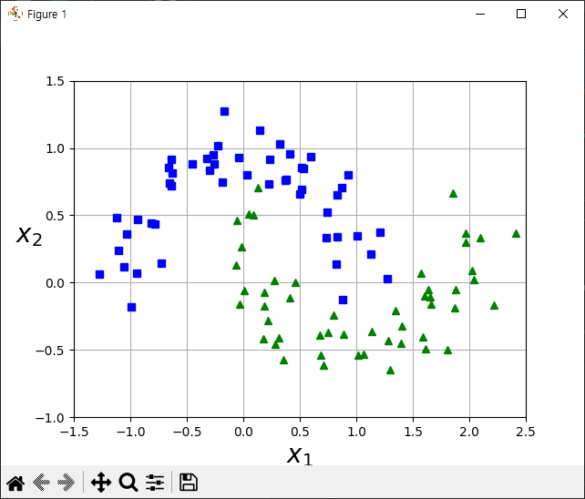
plot_dataset(X, y, [-1.5, 2.5, -1, 1.5])
plt.show()

############################################################################
from sklearn.pipeline import Pipeline

polynomial_svm_clf = Pipeline([
    ('poly_feature',PolynomialFeatures(degree=3)),
    ('scalar',StandardScaler()),
    ('svm_clf',LinearSVC(C=10, random_state=42))
])

polynomial_svm_clf.fit(X,y)



############################################################################

def plot_predictions(clf, axes):
    x0s = np.linspace(axes[0], axes[1], 100)
    x1s = np.linspace(axes[2], axes[3], 100)
    x0, x1 = np.meshgrid(x0s, x1s)
    X = np.c_[x0.ravel(), x1.ravel()]
    y_pred = clf.predict(X).reshape(x0.shape)
    y_decision = clf.decision_function(X).reshape(x0.shape)
    plt.contourf(x0, x1, y_pred, cmap=plt.cm.brg, alpha=0.2)
    plt.contourf(x0, x1, y_decision, cmap=plt.cm.brg, alpha=0.1)

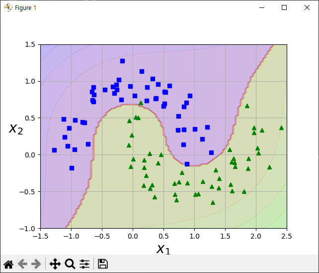
plot_predictions(polynomial_svm_clf, [-1.5, 2.5, -1, 1.5])
plot_dataset(X, y, [-1.5, 2.5, -1, 1.5])
plt.show()

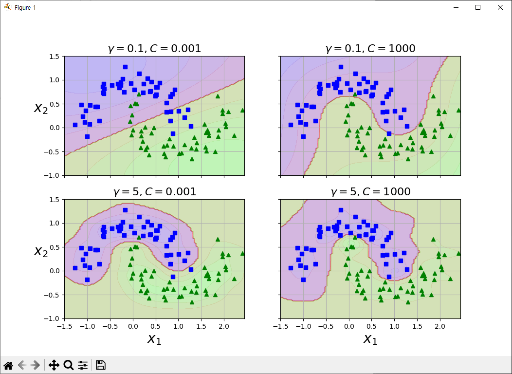
가우시안 커널 계산에서 사용된 Γ 는 가우시안 커널의 폭을 제어하는 매개 변수이다.
Γ 는 가우시안 커널 폭의 역수에 해당한다. 즉 Γ 매개 변수가 하나의 훈련 샘플이 미치는 영향의 범위를 결정한다.
작은 값은 넓은 영역을 뜻하며 큰 값이라면 영향이 미치는 범위가 제한적이다.
C 매개 변수는 선형 모델에서 사용한 것과 비슷한 규제 매개 변수이다. 이 매개 변수는 포인트의 중요도를 제한한다.

from sklearn.svm import SVC
from sklearn.pipeline import Pipeline
from sklearn.preprocessing import StandardScaler
from sklearn.datasets import make_moons
import matplotlib.pyplot as plt
import numpy as np

def plot_predictions(clf, axes):
    x0s = np.linspace(axes[0], axes[1], 100)
    x1s = np.linspace(axes[2], axes[3], 100)
    x0, x1 = np.meshgrid(x0s, x1s)
    X = np.c_[x0.ravel(), x1.ravel()]
    y_pred = clf.predict(X).reshape(x0.shape)
    y_decision = clf.decision_function(X).reshape(x0.shape)
    plt.contourf(x0, x1, y_pred, cmap=plt.cm.brg, alpha=0.2)
    plt.contourf(x0, x1, y_decision, cmap=plt.cm.brg, alpha=0.1)

def plot_dataset(X, y, axes):
    plt.plot(X[:, 0][y==0], X[:, 1][y==0], "bs")
    plt.plot(X[:, 0][y==1], X[:, 1][y==1], "g^")
    plt.axis(axes)
    plt.grid(True, which='both')
    plt.xlabel(r"$x_1$", fontsize=20)
    plt.ylabel(r"$x_2$", fontsize=20, rotation=0)

X, y = make_moons(n_samples=100, noise=0.15, random_state=42)


from sklearn.svm import SVC

gamma1, gamma2 = 0.1, 5
C1, C2 = 0.001, 1000
hyperparams = (gamma1, C1), (gamma1, C2), (gamma2, C1), (gamma2, C2)

svm_clfs = []
for gamma, C in hyperparams:
    rbf_kernel_svm_clf = Pipeline([
            ("scaler", StandardScaler()),
            ("svm_clf", SVC(kernel="rbf", gamma=gamma, C=C))
        ])
    rbf_kernel_svm_clf.fit(X, y)
    svm_clfs.append(rbf_kernel_svm_clf)

fig, axes = plt.subplots(nrows=2, ncols=2, figsize=(10.5, 7), sharex=True, sharey=True)

for i, svm_clf in enumerate(svm_clfs):
    plt.sca(axes[i // 2, i % 2])
    plot_predictions(svm_clf, [-1.5, 2.45, -1, 1.5])
    plot_dataset(X, y, [-1.5, 2.45, -1, 1.5])
    gamma, C = hyperparams[i]
    plt.title(r"$\gamma = {}, C = {}$".format(gamma, C), fontsize=16)
    if i in (0, 1):
        plt.xlabel("")
    if i in (1, 3):
        plt.ylabel("")

plt.show()

하이파라미터 정하기

Grid Search

from sklearn.tree import DecisionTreeClassifier
from sklearn.model_selection import GridSearchCV
import pandas as pd

wine = pd.read_csv('https://bit.ly/wine-date')

data = wine[['alcohol','sugar','pH']].to_numpy()
target = wine['class'].to_numpy()

from sklearn.model_selection import train_test_split

x_train, x_test, y_train, y_test = train_test_split(data, target, test_size=0.2, random_state=42)

params = {'min_impurity_decrease': [0.0001, 0.0002,0.0003,0.0004,0.0005]}
gs = GridSearchCV(DecisionTreeClassifier(random_state=42),
                    params,
                    n_jobs=-1)

gs.fit(x_train, y_train)

dt = gs.best_estimator_
print(gs)
print(dt.score(x_train, y_train))
print(gs.best_params_)
print(gs.cv_results_['mean_test_score'])

GridSearchCV(estimator=DecisionTreeClassifier(random_state=42), n_jobs=-1,
             param_grid={'min_impurity_decrease': [0.0001, 0.0002, 0.0003,
                                                   0.0004, 0.0005]})
0.9615162593804117
{'min_impurity_decrease': 0.0001}
[0.86819297 0.86453617 0.86492226 0.86780891 0.86761605]

import numpy as np
params = {'min_impurity_decrease':np.arange(0.0001,0.001,0.0001),
          'max_depth':range(5,20,1),
          'min_samples_split': range(2, 100, 10)}
gs = GridSearchCV(DecisionTreeClassifier(random_state=42), params, n_jobs=-1)
gs.fit(x_train, y_train)
print(gs.best_params_)
print(np.max(gs.cv_results_['mean_test_score']))

{'max_depth': 14, 'min_impurity_decrease': np.float64(0.0004), 'min_samples_split': 12}
0.8683865773302731

moon 데이터셋에서 max_leaf_node 와 min_samples_split 값을 구하고 accuracy 구하기

import matplotlib.pyplot as plt
import numpy as np
from sklearn.datasets import make_moons
from sklearn.model_selection import GridSearchCV
from sklearn.tree import DecisionTreeClassifier


X, y = make_moons(n_samples=10000, noise=0.15, random_state=42)


from sklearn.model_selection import train_test_split

x_train, x_test, y_train, y_test = train_test_split(X, y, test_size=0.2, random_state=42)

params = {
          'max_leaf_nodes': range(5, 40, 1),
          'min_samples_split': range(2, 100, 10)
          }
gs = GridSearchCV(DecisionTreeClassifier(random_state=42),
                    params,
                    n_jobs=-1)

gs.fit(x_train, y_train)
dt = gs.best_estimator_
y_pred = gs.predict(x_test)
print(y_pred)
print(gs.best_params_)
print('accuracy:',gs.score(x_test, y_pred))

[1 1 0 ... 0 0 0]
{'max_leaf_nodes': 22, 'min_samples_split': 12}
accuracy: 1.0

import pandas as pd
import numpy as np
from sklearn.model_selection import GridSearchCV
from sklearn.pipeline import Pipeline
from sklearn.preprocessing import StandardScaler


train = pd.read_csv('https://raw.githubusercontent.com/wikibook/machine-learning/2.0/data/csv/basketball_train.csv')
test = pd.read_csv('https://raw.githubusercontent.com/wikibook/machine-learning/2.0/data/csv/basketball_test.csv')
train.info()
print(train)


x_train = train[['3P','BLK']]
y_train = train['Pos']
x_test = test[['3P','BLK']]
y_test = test['Pos']

from sklearn.svm import SVC
from sklearn.metrics import accuracy_score

def svc_param_selection(x,y):
    svm_parameters = [
        {'kernel':['rbf'],
         'gamma':[0.00001,0.0001,0.001,0.1,1],
         'C':[0.01,0.1,1,10,100]}

    ]
    clf = GridSearchCV(SVC(), svm_parameters, n_jobs=-1)
    clf.fit(x, y.values.ravel())
    print(clf.best_params_)
    return clf

clf = svc_param_selection(x_train,y_train)
y_pred = clf.predict(x_test)
print('accuracy:', accuracy_score(y_test,y_pred))

comparison = pd.DataFrame({'prediction':y_pred, 'truth':y_test.values.ravel()})
print(comparison)

<class 'pandas.core.frame.DataFrame'>
RangeIndex: 80 entries, 0 to 79
Data columns (total 5 columns):
 #   Column  Non-Null Count  Dtype  
---  ------  --------------  -----  
 0   Player  80 non-null     object 
 1   Pos     80 non-null     object 
 2   3P      80 non-null     float64
 3   TRB     80 non-null     float64
 4   BLK     80 non-null     float64
dtypes: float64(3), object(2)
memory usage: 3.2+ KB
                 Player Pos   3P  TRB  BLK
0      Denzel Valentine  SG  1.3  2.6  0.1
1           Kyle Korver  SG  2.4  2.8  0.3
2          Troy Daniels  SG  2.1  1.5  0.1
3          Tim Hardaway  SG  1.9  2.8  0.2
4        Dewayne Dedmon   C  0.0  6.5  0.8
..                  ...  ..  ...  ...  ...
75       Victor Oladipo  SG  1.9  4.3  0.3
76  Willie Cauley-Stein   C  0.0  4.5  0.6
77          Brook Lopez   C  1.8  5.4  1.7
78      Josh Richardson  SG  1.4  3.2  0.7
79         Lou Williams  SG  2.0  2.5  0.2

[80 rows x 5 columns]
{'C': 0.1, 'gamma': 1, 'kernel': 'rbf'}
accuracy: 1.0
   prediction truth
0           C     C
1          SG    SG
2           C     C
3          SG    SG
4           C     C
5           C     C
6           C     C
7          SG    SG
8          SG    SG
9           C     C
10         SG    SG
11          C     C
12         SG    SG
13          C     C
14          C     C
15         SG    SG
16         SG    SG
17          C     C
18         SG    SG
19          C     C

앙상블

앙상블(ensemble)은 머신러닝 모델을 연결하여 더 강력한 모델을 만드는 기법이다.
대표적인 앙상블 모델은 배깅(bagging) 과 부스팅 (boosting) 이 있다.
두 모델은 기본요소로 결정 트리를 사용한다.
배깅을 사용하는 대표적인 모델은 랜덤 포레스트(random forest)이다.
부스팅을 사용하는 대표적인 모델은 그래디어트 부스팅(gradient boosting)이다.

Bagging(Bootstrap Aggregation)은 샘플을 여러 번 뽑아 (Bootstrap) 각 모델을 학습시켜 결과물을 집계(Aggregation) 하는 방법이다.

배깅은 무작위로 훈련 데이터 셋을 잘게 나눈 후 나누어진 훈련 데이터 셋을 여러 개의 모델에 할당하여 학습시킨다.

배깅은 중복을 허용하며 훈련 데이터 셋을 나누는데 통계학에서는 이 방법을 부트스트랩, 중복이 허용된 리샘플링이라고 한다.

랜덤 포레스트는 배깅 방법을 결정 트리를 이용한 앙상블 방법이다.

사용할 때는 baggingClassifier 에 DecisionTreeClassifier 을 넣어 만드는 대신 결정 트리에 최적화 되어 있는 RandomForestClassifier를 사용할 수 있다.

랜덤 포레스트는 성능이 매우 뛰어나고 매개변수 튜닝을 많이 하지 않아도 잘 작동하며, 데이터의 스케일을 맞출 필요도 없다.


from sklearn.datasets import make_moons
from sklearn.model_selection import train_test_split

from day3.gridSearchEx3 import svm_clfs
from day3.gridSearchEx3answer import y_pred

x, y = make_moons(n_samples=500, noise=0.30, random_state=42)
x_train, x_test, y_train, y_test = train_test_split(x,y,random_state=42)

from sklearn.linear_model import LogisticRegression
from sklearn.svm import SVC
from sklearn.ensemble import RandomForestClassifier
from sklearn.ensemble import VotingClassifier

log_clf = LogisticRegression(random_state=42)
rnd_Clf = RandomForestClassifier(n_estimators=100, random_state=42)
svm_clf = SVC(random_state=42)

voting_clf = VotingClassifier(
    estimators=[('lr',log_clf),('rf',rnd_Clf),('svc',svm_clf)],
    voting='hard'
)

from sklearn.metrics import accuracy_score
for clf in (log_clf, rnd_Clf, svm_clf, voting_clf):
    clf.fit(x_train, y_train)
    y_pred = clf.predict(x_test)
    print(clf.__class__.__name__, accuracy_score(y_test, y_pred))
    
# 간접 투표
log_clf = LogisticRegression(random_state=42)
rnd_clf = RandomForestClassifier(n_estimators=100, random_state=42)
svm_clf = SVC(probability=True, random_state=42)

voting_clf = VotingClassifier(
    estimators=[('lr',log_clf),('rf',rnd_clf),('svc',svm_clf)],
    voting='hard'
)

from sklearn.metrics import accuracy_score
for clf in (log_clf, rnd_clf, svm_clf, voting_clf):
    clf.fit(x_train, y_train)
    y_pred = clf.predict(x_test)
    print(clf.__class__.__name__, accuracy_score(y_test, y_pred))

LogisticRegression 0.864
RandomForestClassifier 0.896
SVC 0.896
VotingClassifier 0.912

LogisticRegression 0.864
RandomForestClassifier 0.896
SVC 0.896
VotingClassifier 0.912

from sklearn.datasets import load_digits
from sklearn.model_selection import train_test_split
from sklearn.tree import DecisionTreeClassifier
from sklearn.svm import SVC
from sklearn.neighbors import KNeighborsClassifier
from sklearn.ensemble import VotingClassifier
from sklearn.metrics import accuracy_score
import numpy as np


np.random.seed(5)

mnist = load_digits()
print(mnist.keys())
print(mnist.DESCR)
print(mnist.data.shape)
print(mnist.target)

x_train, x_test, y_train, y_test = train_test_split(mnist.data, mnist.target,
                                                    test_size=0.2, random_state=42)

dtree = DecisionTreeClassifier(max_depth=8, random_state=42)
dtree = dtree.fit(x_train, y_train)
dtree_predict = dtree.predict(x_test)

knn = KNeighborsClassifier(n_neighbors=299)
knn = knn.fit(x_train, y_train)
knn_predict = knn.predict(x_test)


svm = SVC(C=0.1, gamma = 0.003, probability=True, random_state=35)
svm = svm.fit(x_train, y_train)
svm_predict = svm.predict(x_test)

print('accuracy')
print('dtree: ', accuracy_score(y_test, dtree_predict))
print('knn :', accuracy_score(y_test, knn_predict))
print('svm :', accuracy_score(y_test, svm_predict))

voting_clf = VotingClassifier(
    estimators=[
        ('dt',dtree),('knn',knn),('svm',svm)
    ],
    voting='hard'
)

hard_voting_predicted = voting_clf.fit(x_train,y_train).predict(x_test)
print('voting(hard): ', accuracy_score(y_test, hard_voting_predicted))

voting_clf2 = VotingClassifier(
    estimators=[
        ('dt',dtree),('knn',knn),('svm',svm)
    ],
    voting='soft'
)

soft_voting_predicted = voting_clf2.fit(x_train,y_train).predict(x_test)
print('voting(soft): ', accuracy_score(y_test, soft_voting_predicted))

dict_keys(['data', 'target', 'frame', 'feature_names', 'target_names', 'images', 'DESCR'])
.. _digits_dataset:

Optical recognition of handwritten digits dataset
--------------------------------------------------

**Data Set Characteristics:**

:Number of Instances: 1797
:Number of Attributes: 64
:Attribute Information: 8x8 image of integer pixels in the range 0..16.
:Missing Attribute Values: None
:Creator: E. Alpaydin (alpaydin '@' boun.edu.tr)
:Date: July; 1998

This is a copy of the test set of the UCI ML hand-written digits datasets
https://archive.ics.uci.edu/ml/datasets/Optical+Recognition+of+Handwritten+Digits

The data set contains images of hand-written digits: 10 classes where
each class refers to a digit.

Preprocessing programs made available by NIST were used to extract
normalized bitmaps of handwritten digits from a preprinted form. From a
total of 43 people, 30 contributed to the training set and different 13
to the test set. 32x32 bitmaps are divided into nonoverlapping blocks of
4x4 and the number of on pixels are counted in each block. This generates
an input matrix of 8x8 where each element is an integer in the range
0..16. This reduces dimensionality and gives invariance to small
distortions.

For info on NIST preprocessing routines, see M. D. Garris, J. L. Blue, G.
T. Candela, D. L. Dimmick, J. Geist, P. J. Grother, S. A. Janet, and C.
L. Wilson, NIST Form-Based Handprint Recognition System, NISTIR 5469,
1994.

.. dropdown:: References

  - C. Kaynak (1995) Methods of Combining Multiple Classifiers and Their
    Applications to Handwritten Digit Recognition, MSc Thesis, Institute of
    Graduate Studies in Science and Engineering, Bogazici University.
  - E. Alpaydin, C. Kaynak (1998) Cascading Classifiers, Kybernetika.
  - Ken Tang and Ponnuthurai N. Suganthan and Xi Yao and A. Kai Qin.
    Linear dimensionalityreduction using relevance weighted LDA. School of
    Electrical and Electronic Engineering Nanyang Technological University.
    2005.
  - Claudio Gentile. A New Approximate Maximal Margin Classification
    Algorithm. NIPS. 2000.

(1797, 64)
[0 1 2 ... 8 9 8]
accuracy
dtree:  0.8361111111111111
knn : 0.8472222222222222
svm : 0.8972222222222223
voting(hard):  0.9138888888888889
voting(soft):  0.9055555555555556

부스팅은 가중치를 활용하여 약 분류기를 강 분류기로 만드는 방법이다.
배깅은 Deicison Tree 1 과 Decision Tree 2 가 서로 독립적으로 결과를 예측한다. 그러나 부스팅은 모델 간 결정에 영향을 준다. 처음 모델이 예측을 하면 그 예측 결과에 따라 데이터에 가중치가 부여되고, 부여된 가중치가 다음 모델에 영향을 준다. 즉 잘못 분류된 데이터에 집중하여 새로운 분류 규칙을 만드는 단계를 반복한다.

그래디언트 부스팅은 여러 개의 결정 트리를 묶어 강력한 모델을 만든다.
랜덤 포레스트와는 달리 그래디언트 부스팅은 이전 트리의 오차를 보안하는 방식으로 순차적 트리를 만든다.
기본적으로 그래디언트 부스팅은 강력한 사전치기가 사용되어 메모리를 작게 사용하고 예측도 빠르다.
각각의 트리는 데이터의 일부에 대해서만 예측을 잘 수행할 수 있어서 트리가 많이 추가 될수록 성능이 좋아진다.

bagging , pasting

from sklearn.datasets import make_moons
from sklearn.model_selection import train_test_split

x, y = make_moons(n_samples=500, noise=0.30, random_state=42)
x_train, x_test, y_train, y_test = train_test_split(x,y,random_state=42)

from sklearn.ensemble import BaggingClassifier
from sklearn.tree import DecisionTreeClassifier
from sklearn.metrics import accuracy_score

bag_clf = BaggingClassifier(
    DecisionTreeClassifier(), n_estimators=500, max_samples=100,
    bootstrap=True, random_state=42
)

bag_clf.fit(x_train,y_train)
y_pred = bag_clf.predict(x_test)
print('bagging accuracy: ',accuracy_score(y_test,y_pred))

bag_clf2 = BaggingClassifier(
    DecisionTreeClassifier(), n_estimators=500, max_samples=100,
    bootstrap=False, random_state=42
)

bag_clf2.fit(x_train,y_train)
y_pred = bag_clf2.predict(x_test)
print('pasting accuracy: ',accuracy_score(y_test,y_pred))

bagging accuracy:  0.904
pasting accuracy:  0.92

AdaBoostClassifier


from sklearn.datasets import make_moons
from sklearn.metrics import accuracy_score
from sklearn.model_selection import train_test_split
from sklearn.tree import DecisionTreeClassifier

x, y = make_moons(n_samples=500, noise=0.30, random_state=42)
x_train, x_test, y_train, y_test = train_test_split(x,y,random_state=42)

from sklearn.ensemble import AdaBoostClassifier

ada_clf = AdaBoostClassifier(DecisionTreeClassifier(max_depth=1),
                             n_estimators=300,
                             random_state=42,
                             learning_rate=0.3)
ada_clf.fit(x_train, y_train)
y_pred = ada_clf.predict(x_test)
print(accuracy_score(y_test, y_pred))

0.904

DecisionTreeRegressor 및 GradientBoostingRegressor


from sklearn.datasets import make_moons
from sklearn.metrics import accuracy_score
from sklearn.model_selection import train_test_split
from sklearn.tree import DecisionTreeClassifier

# x, y = make_moons(n_samples=500, noise=0.30, random_state=42)
# x_train, x_test, y_train, y_test = train_test_split(x,y,random_state=42)
#
# from sklearn.ensemble import AdaBoostClassifier
#
# ada_clf = AdaBoostClassifier(DecisionTreeClassifier(max_depth=1),
#                              n_estimators=300,
#                              random_state=42,
#                              learning_rate=0.3)
# ada_clf.fit(x_train, y_train)
# y_pred = ada_clf.predict(x_test)
# print(accuracy_score(y_test, y_pred))

from sklearn.tree import DecisionTreeRegressor
import numpy as np


x = np.random.rand(100,1) -0.5
y = 3 * x[:,0]**2 + 0.05 + np.random.randn(100)

tree_reg1 = DecisionTreeRegressor(max_depth=2, random_state=42)
tree_reg1.fit(x,y)
y2 = y - tree_reg1.predict(x)

tree_reg2 = DecisionTreeRegressor(max_depth=2, random_state=42)
tree_reg2.fit(x,y2)
y3 = y2 - tree_reg2.predict(x)

tree_reg3 = DecisionTreeRegressor(max_depth=2, random_state=42)
tree_reg3.fit(x,y3)

x_new = np.array([[0.8]])

y_pred = sum((tree.predict(x_new) for tree in (tree_reg1, tree_reg2, tree_reg3)))
print(y_pred)

from sklearn.ensemble import GradientBoostingRegressor
gbrt = GradientBoostingRegressor(max_depth=2, n_estimators=300, learning_rate=0.8)
gbrt.fit(x,y)
gbrt.predict(x)

[0.81747447]

import pandas as pd
from sklearn.datasets import load_breast_cancer
from sklearn.model_selection import train_test_split
from sklearn.tree import DecisionTreeClassifier
from sklearn.neighbors import KNeighborsClassifier
from sklearn.linear_model import LogisticRegression


cancer = load_breast_cancer()
print(cancer.target)

x_train, x_test, y_train, y_test = train_test_split(cancer.data, cancer.target, random_state=0)
x_train, x_val, y_train, y_val = train_test_split(x_train, y_train, random_state=10)

model1 = DecisionTreeClassifier()
model1.fit(x_train, y_train)
val_pred1 = model1.predict(x_val)
test_pred1 = model1.predict(x_test)

val_pred1 = pd.DataFrame(val_pred1)
test_pred1 = pd.DataFrame(test_pred1)

model2 = KNeighborsClassifier()
model2.fit(x_train, y_train)
val_pred2 = model2.predict(x_val)
test_pred2 = model2.predict(x_test)

val_pred2 = pd.DataFrame(val_pred2)
test_pred2 = pd.DataFrame(test_pred2)

x_val = pd.DataFrame(x_val)
x_test = pd.DataFrame(x_test)

df_val = pd.concat([x_val, val_pred1, val_pred2], axis=1)
df_test = pd.concat([x_test, test_pred1, test_pred2], axis=1)

model = LogisticRegression(max_iter=5000)
model.fit(df_val, y_val)
print('accuracy :', model.score(df_test,y_test))

[0 0 0 0 0 0 0 0 0 0 0 0 0 0 0 0 0 0 0 1 1 1 0 0 0 0 0 0 0 0 0 0 0 0 0 0 0
 1 0 0 0 0 0 0 0 0 1 0 1 1 1 1 1 0 0 1 0 0 1 1 1 1 0 1 0 0 1 1 1 1 0 1 0 0
 1 0 1 0 0 1 1 1 0 0 1 0 0 0 1 1 1 0 1 1 0 0 1 1 1 0 0 1 1 1 1 0 1 1 0 1 1
 1 1 1 1 1 1 0 0 0 1 0 0 1 1 1 0 0 1 0 1 0 0 1 0 0 1 1 0 1 1 0 1 1 1 1 0 1
 1 1 1 1 1 1 1 1 0 1 1 1 1 0 0 1 0 1 1 0 0 1 1 0 0 1 1 1 1 0 1 1 0 0 0 1 0
 1 0 1 1 1 0 1 1 0 0 1 0 0 0 0 1 0 0 0 1 0 1 0 1 1 0 1 0 0 0 0 1 1 0 0 1 1
 1 0 1 1 1 1 1 0 0 1 1 0 1 1 0 0 1 0 1 1 1 1 0 1 1 1 1 1 0 1 0 0 0 0 0 0 0
 0 0 0 0 0 0 0 1 1 1 1 1 1 0 1 0 1 1 0 1 1 0 1 0 0 1 1 1 1 1 1 1 1 1 1 1 1
 1 0 1 1 0 1 0 1 1 1 1 1 1 1 1 1 1 1 1 1 1 0 1 1 1 0 1 0 1 1 1 1 0 0 0 1 1
 1 1 0 1 0 1 0 1 1 1 0 1 1 1 1 1 1 1 0 0 0 1 1 1 1 1 1 1 1 1 1 1 0 0 1 0 0
 0 1 0 0 1 1 1 1 1 0 1 1 1 1 1 0 1 1 1 0 1 1 0 0 1 1 1 1 1 1 0 1 1 1 1 1 1
 1 0 1 1 1 1 1 0 1 1 0 1 1 1 1 1 1 1 1 1 1 1 1 0 1 0 0 1 0 1 1 1 1 1 0 1 1
 0 1 0 1 1 0 1 0 1 1 1 1 1 1 1 1 0 0 1 1 1 1 1 1 0 1 1 1 1 1 1 1 1 1 1 0 1
 1 1 1 1 1 1 0 1 0 1 1 0 1 1 1 1 1 0 0 1 0 1 0 1 1 1 1 1 0 1 1 0 1 0 1 0 0
 1 1 1 0 1 1 1 1 1 1 1 1 1 1 1 0 1 0 0 1 1 1 1 1 1 1 1 1 1 1 1 1 1 1 1 1 1
 1 1 1 1 1 1 1 0 0 0 0 0 0 1]
accuracy : 0.9370629370629371

짬그브

+AI to AI+

이전 포스트

머신러닝 (지도학습)

다음 포스트