전처리 방법

비지도학습

비지도 학습에는 비지도 변환(unsupervised transformation) 과 군집(clustering) 이 있다.

비지도 변환은 데이터를 새롭게 표현하여 사람이나 다른 머신러닝 알고리즘이 원래 데이터보다 쉽게 해석할 수 있도록 만드는 알고리즘이다.

많은 고차원 데이터를 특성의 수를 줄이면서 꼭 필요한 특징을 포함한 데이터로 표현하는 방법인 차원 축소(dimensionality reduction)의 대표적 예는 시각화를 위해 데이터셋을 2차원으로 변경하는 경우이다.
비지도 변환으로 데이터를 구성하는 단위나 성분을 검색하여 많은 텍스트 문서에서 주제를 추출할 수 있다.
소셜 미디어에서 선거, 총기 규제, 팝스타 같은 주제로 일어나는 토론을 추적할 때 사용 가능하다.

군집은 데이터를 비슷한 것끼리 그룹으로 묶는 작업이다.

소셜 미디어 사이트에 사진을 업로드 하는 경우와 업로드한 사진을 분류하려면 같은 사람이 찍힌 사진을 같은 그룹으로 묶을 수 있으나 사이트는 사진에 찍힌 사람이 누군지, 전체 사진 앨범에 얼마나 많은 사람이 있는지 알지 못한다. 이때 가능한 방법은 사진에 나타난 모든 얼굴을 추출해서 비슷한 얼굴로 그룹 짓는 것이다.

비지도 학습에서 가장 어려운 일은 알고리즘이 뭔가 유용한 것을 학습했는지 평가하는 것이다.

비지도 학습은 보통 레이블이 없는 데이터에 적용하기 때문에 무엇이 올바른 출력인지 모른다는 단점이 있다.

비지도 학습의 결과를 평가하기 위해서는 직접 확인하는 것이 유일한 방법일 때가 많다.

비지도 학습 알고리즘은 데이터 과학자가 데이터를 더 잘 이해하고 싶을 때 탐색적 분석 단계에서 많이 사용된다.

비지도 학습은 지도 학습의 전처리 단계에서도 사용된다. 그 이유는 비지도 학습의 결과로 새롭게 표현된 데이터를 사용해 학습하면 지도 학습의 정확도가 좋아지기도 하며 메모리와 시간을 절약할 수 있기 때문이다.

from sklearn.preprocessing import StandardScaler
import numpy as np

features = np.array([[-500.5],
                     [-100.1],
                     [0],
                     [900.9]])

ss_scaler = StandardScaler()
scaled_feature1 = ss_scaler.fit_transform(features)
print(scaled_feature1)
print()

from sklearn.preprocessing import RobustScaler
r_scaler = RobustScaler()
scaled_feature2 = r_scaler.fit_transform(features)
print(scaled_feature2)
print()

from sklearn.preprocessing import MinMaxScaler
minmax_scaler = MinMaxScaler()
scaled_feature3 = minmax_scaler.fit_transform(features)
print(scaled_feature3)
print()

from sklearn.preprocessing import Normalizer

features = np.array([[0.5,0.5],
                     [1.1,3.4],
                     [1.5,20.2],
                     [1.63,34.4],
                     [10.9,3.3]])

n_scaler = Normalizer(norm='l1')
scaled_feature4 = n_scaler.fit_transform(features)
print(scaled_feature4)

---

[[-1.12362353]
 [-0.34197238]
 [-0.14655959]
 [ 1.6121555 ]]

[[-1.05882353]
 [-0.11764706]
 [ 0.11764706]
 [ 2.23529412]]

[[0.        ]
 [0.28571429]
 [0.35714286]
 [1.        ]]

[[0.5        0.5       ]
 [0.24444444 0.75555556]
 [0.06912442 0.93087558]
 [0.04524008 0.95475992]
 [0.76760563 0.23239437]]
 

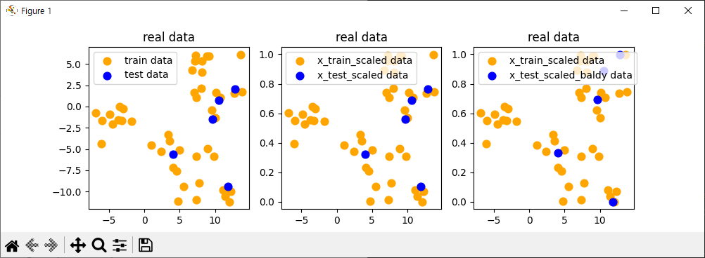
from sklearn.model_selection import train_test_split
from sklearn.preprocessing import MinMaxScaler
from sklearn.datasets import make_blobs
import matplotlib.pyplot as plt


x , _ = make_blobs(n_samples=50, centers=5, random_state=4, cluster_std=2)
x_train, x_test = train_test_split(x, random_state=5, test_size=0.1)

fig, axes = plt.subplots(1,3,figsize=(10,3))
axes[0].scatter(x_train[:,0], x_train[:,1], c='orange', label='train data', s=60)
axes[0].scatter(x_test[:,0], x_test[:,1], c='blue', label='test data', s=60)
axes[0].legend(loc='upper left')
axes[0].set_title('real data')

scaler = MinMaxScaler()
scaler.fit(x_train)
x_train_scaled = scaler.transform(x_train)
x_test_scaled = scaler.transform(x_test)

axes[1].scatter(x_train[:,0], x_train_scaled[:,1], c='orange', label='x_train_scaled data', s=60)
axes[1].scatter(x_test[:,0], x_test_scaled[:,1], c='blue', label='x_test_scaled data', s=60)
axes[1].legend(loc='upper left')
axes[1].set_title('real data')

test_scaler = MinMaxScaler()
test_scaler.fit(x_test)
x_test_scaled_baldy = test_scaler.transform(x_test)

axes[2].scatter(x_train[:,0], x_train_scaled[:,1], c='orange', label='x_train_scaled data', s=60)
axes[2].scatter(x_test[:,0], x_test_scaled_baldy[:,1], c='blue', label='x_test_scaled_baldy data', s=60)
axes[2].legend(loc='upper left')
axes[2].set_title('real data')


plt.show()