quiz 1번
from sklearn.datasets import fetch_openml
import ssl
ssl._create_default_https_context = ssl._create_unverified_context
from sklearn.model_selection import GridSearchCV
from sklearn.tree import DecisionTreeClassifier
from sklearn.neighbors import KNeighborsClassifier
mnist = fetch_openml('mnist_784', as_frame=False)
x, y = mnist.data, mnist.target
# print(mnist)
import matplotlib.pyplot as plt
import numpy as np
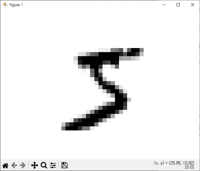
def plot_digit(image_data):
image = image_data.reshape(28, 28)
plt.imshow(image, cmap='binary')
plt.axis('off')
some_digit = x[0]
plot_digit(some_digit)
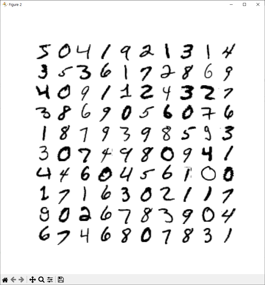
plt.figure(figsize=(9,9))
for idx, image_data in enumerate(x[:100]):
plt.subplot(10,10, idx+1)
plot_digit(image_data)
plt.subplots_adjust(wspace=0,hspace=0)
plt.show()
knn_clf = KNeighborsClassifier()
params = [{'n_neighbors':range(3,8,1), 'weights':['uniform','distance']}]
from sklearn.model_selection import train_test_split
x_train, x_test, y_train, y_test= train_test_split(x[:10000], y[:10000], test_size=0.2, random_state=0)
grid_search = GridSearchCV(knn_clf, params, cv=5)
grid_search.fit(x_train, y_train)
print(grid_search.best_score_)
print(grid_search.best_params_)
print()
bestmodel = grid_search.best_estimator_
bestmodel.fit(x_train,y_train)
print(bestmodel.score(x_test,y_test))
0.94525
{'n_neighbors': 4, 'weights': 'distance'}

0.9495
quiz 2번
import pandas as pd


passengers = pd.read_csv('titanic_data.csv')
passengers.info()
print(passengers['Pclass'])
print()

dummies = pd.get_dummies(passengers['Pclass'])
print(dummies)
print()
del passengers['Pclass']
passengers = pd.concat([passengers, dummies], axis=1, join='inner')
passengers.info()
print()
print(passengers['Sex'])
'''
1. age 누락값을 평균으로 채움

2. Sex의 male = > 0, female = > 1

3. 1 => FirstClass  2 => SecondClass 3 => EtcClass

4. Sex,Age,FirstClass,SecondClass,EtcClass 를 특성 데이터로 이용해서 Survived 를 예측하는 모델을 구성

5. LogisticRegression 을 이용

6. 데이터 train, test 비율 8 : 2

7. 특성 데이터(x_train, x_test)는 standarScaler를 이용해 스케일 작업을 한다

8. 학습 완료 후
kim = np.array([0.0,20.0,0.0,0.0,1.0])
hyo = np.array([1.0,17.0,1.0,0.0,0.0])
choi = np.array([0.0,32.0,0.0,1.0,0.0])

'''

# 1. age 누락값을 평균으로 채움

meanage = passengers['Age'].mean()
print(meanage)
passengers.fillna({'Age':int(meanage)},inplace=True)
print(passengers['Age'])

# 2. Sex의 male = > 0, female = > 1
passengers['Sex'] = passengers['Sex'].map({'male':0,'female':1})
print(passengers['Sex'])

# 3. 1 => FirstClass  2 => SecondClass 3 => EtcClass
passengers.rename(columns={1:'FirstClass',2:'SecondClass',3:'EtcClass'}, inplace=True)
passengers.info()

# 4. Sex,Age,FirstClass,SecondClass,EtcClass 를 특성 데이터로 이용해서 Survived 를 예측하는 모델을 구성
# 5. LogisticRegression 을 이용
# 6. 데이터 train, test 비율 8 : 2

x_input = passengers.loc[:,['Sex','Age','FirstClass','SecondClass','EtcClass']].values
x_target = passengers['Survived'].to_numpy()
print(x_input.shape)

from sklearn.model_selection import train_test_split

train_input, test_input, train_target, test_target = train_test_split(
    x_input, x_target, test_size=0.2, random_state=42
)

from sklearn.preprocessing import StandardScaler

ss = StandardScaler()
ss.fit(train_input)
train_scaled = ss.transform(train_input)
test_scaled = ss.transform(test_input)

from sklearn.linear_model import LogisticRegression

import numpy as np

kim = np.array([0.0,20.0,0.0,0.0,1.0])
hyo = np.array([1.0,17.0,1.0,0.0,0.0])
choi = np.array([0.0,32.0,0.0,1.0,0.0])


A = np.stack((kim,hyo,choi),axis=0)
A_scaled = ss.transform(A)

lr = LogisticRegression()
lr.fit(train_scaled, train_target)

print('train data accuracy: ', lr.score(train_scaled, train_target))
print('test data accuracy: ', lr.score(test_scaled, test_target))


y_pred = lr.predict(A_scaled)
print(y_pred)
<class 'pandas.core.frame.DataFrame'>
RangeIndex: 891 entries, 0 to 890
Data columns (total 12 columns):
 #   Column       Non-Null Count  Dtype
---  ------       --------------  -----
 0   PassengerId  891 non-null    int64
 1   Survived     891 non-null    int64
 2   Pclass       891 non-null    int64
 3   Name         891 non-null    object
 4   Sex          891 non-null    object
 5   Age          714 non-null    float64
 6   SibSp        891 non-null    int64
 7   Parch        891 non-null    int64
 8   Ticket       891 non-null    object
 9   Fare         891 non-null    float64
 10  Cabin        204 non-null    object
 11  Embarked     889 non-null    object
dtypes: float64(2), int64(5), object(5)
memory usage: 83.7+ KB
0      3
1      1
2      3
3      1
4      3
      ..
886    2
887    1
888    3
889    1
890    3
Name: Pclass, Length: 891, dtype: int64

         1      2      3
0    False  False   True
1     True  False  False
2    False  False   True
3     True  False  False
4    False  False   True
..     ...    ...    ...
886  False   True  False
887   True  False  False
888  False  False   True
889   True  False  False
890  False  False   True

[891 rows x 3 columns]

<class 'pandas.core.frame.DataFrame'>
RangeIndex: 891 entries, 0 to 890
Data columns (total 14 columns):
 #   Column       Non-Null Count  Dtype
---  ------       --------------  -----
 0   PassengerId  891 non-null    int64
 1   Survived     891 non-null    int64
 2   Name         891 non-null    object
 3   Sex          891 non-null    object
 4   Age          714 non-null    float64
 5   SibSp        891 non-null    int64
 6   Parch        891 non-null    int64
 7   Ticket       891 non-null    object
 8   Fare         891 non-null    float64
 9   Cabin        204 non-null    object
 10  Embarked     889 non-null    object
 11  1            891 non-null    bool
 12  2            891 non-null    bool
 13  3            891 non-null    bool
dtypes: bool(3), float64(2), int64(4), object(5)
memory usage: 79.3+ KB

0        male
1      female
2      female
3      female
4        male
        ...
886      male
887    female
888    female
889      male
890      male
Name: Sex, Length: 891, dtype: object
29.69911764705882
0      22.0
1      38.0
2      26.0
3      35.0
4      35.0
       ...
886    27.0
887    19.0
888    29.0
889    26.0
890    32.0
Name: Age, Length: 891, dtype: float64
0      0
1      1
2      1
3      1
4      0
      ..
886    0
887    1
888    1
889    0
890    0
Name: Sex, Length: 891, dtype: int64
<class 'pandas.core.frame.DataFrame'>
RangeIndex: 891 entries, 0 to 890
Data columns (total 14 columns):
 #   Column       Non-Null Count  Dtype
---  ------       --------------  -----
 0   PassengerId  891 non-null    int64
 1   Survived     891 non-null    int64
 2   Name         891 non-null    object
 3   Sex          891 non-null    int64
 4   Age          891 non-null    float64
 5   SibSp        891 non-null    int64
 6   Parch        891 non-null    int64
 7   Ticket       891 non-null    object
 8   Fare         891 non-null    float64
 9   Cabin        204 non-null    object
 10  Embarked     889 non-null    object
 11  FirstClass   891 non-null    bool
 12  SecondClass  891 non-null    bool
 13  EtcClass     891 non-null    bool
dtypes: bool(3), float64(2), int64(5), object(4)
memory usage: 79.3+ KB
(891, 5)
train data accuracy:  0.7949438202247191
test data accuracy:  0.8044692737430168
[0 1 0]
quiz 3번
from sklearn.datasets import load_wine
from sklearn.svm import LinearSVC

wine = load_wine(as_frame=True)
print(wine)
print(wine.data)
print(type(wine.data))
print(wine.DESCR)


from sklearn.model_selection import train_test_split

x_train, x_test, y_train, y_test = train_test_split(wine.data, wine.target,random_state=42)
# (scaler LinearSVC) pipeline

from sklearn.pipeline import Pipeline
from sklearn.svm import LinearSVC
from sklearn.preprocessing import StandardScaler, PolynomialFeatures

svm_clf = Pipeline([
    ('scalar',StandardScaler()),
    ('svm_clf',LinearSVC(C=10, random_state=42))
])

svm_clf.fit(x_train, y_train)
print(svm_clf.predict(x_train[:10]))   # 예측 값 10번째 까지
print(svm_clf.score(x_test,y_test))  # accuracy
{'data':      alcohol  malic_acid   ash  ...   hue  od280/od315_of_diluted_wines  proline
0      14.23        1.71  2.43  ...  1.04                          3.92   1065.0
1      13.20        1.78  2.14  ...  1.05                          3.40   1050.0
2      13.16        2.36  2.67  ...  1.03                          3.17   1185.0
3      14.37        1.95  2.50  ...  0.86                          3.45   1480.0
4      13.24        2.59  2.87  ...  1.04                          2.93    735.0
..       ...         ...   ...  ...   ...                           ...      ...
173    13.71        5.65  2.45  ...  0.64                          1.74    740.0
174    13.40        3.91  2.48  ...  0.70                          1.56    750.0
175    13.27        4.28  2.26  ...  0.59                          1.56    835.0
176    13.17        2.59  2.37  ...  0.60                          1.62    840.0
177    14.13        4.10  2.74  ...  0.61                          1.60    560.0

[178 rows x 13 columns], 'target': 0      0
1      0
2      0
3      0
4      0
      ..
173    2
174    2
175    2
176    2
177    2
Name: target, Length: 178, dtype: int64, 'frame':      alcohol  malic_acid   ash  ...  od280/od315_of_diluted_wines  proline  target
0      14.23        1.71  2.43  ...                          3.92   1065.0       0
1      13.20        1.78  2.14  ...                          3.40   1050.0       0
2      13.16        2.36  2.67  ...                          3.17   1185.0       0
3      14.37        1.95  2.50  ...                          3.45   1480.0       0
4      13.24        2.59  2.87  ...                          2.93    735.0       0
..       ...         ...   ...  ...                           ...      ...     ...
173    13.71        5.65  2.45  ...                          1.74    740.0       2
174    13.40        3.91  2.48  ...                          1.56    750.0       2
175    13.27        4.28  2.26  ...                          1.56    835.0       2
176    13.17        2.59  2.37  ...                          1.62    840.0       2
177    14.13        4.10  2.74  ...                          1.60    560.0       2

[178 rows x 14 columns], 'target_names': array(['class_0', 'class_1', 'class_2'], dtype='<U7'), 'DESCR': '.. _wine_dataset:\n\nWine recognition dataset\n------------------------\n\n**Data Set Characteristics:**\n\n:Number of Instances: 178\n:Number of Attributes: 13 numeric, predictive attributes and the class\n:Attribute Information:\n    - Alcohol\n    - Malic acid\n    - Ash\n    - Alcalinity of ash\n    - Magnesium\n    - Total phenols\n    - Flavanoids\n    - Nonflavanoid phenols\n    - Proanthocyanins\n    - Color intensity\n    - Hue\n    - OD280/OD315 of diluted wines\n    - Proline\n    - class:\n        - class_0\n        - class_1\n        - class_2\n\n:Summary Statistics:\n\n============================= ==== ===== ======= =====\n                                Min   Max   Mean     SD\n============================= ==== ===== ======= =====\nAlcohol:                      11.0  14.8    13.0   0.8\nMalic Acid:                   0.74  5.80    2.34  1.12\nAsh:                          1.36  3.23    2.36  0.27\nAlcalinity of Ash:            10.6  30.0    19.5   3.3\nMagnesium:                    70.0 162.0    99.7  14.3\nTotal Phenols:                0.98  3.88    2.29  0.63\nFlavanoids:                   0.34  5.08    2.03  1.00\nNonflavanoid Phenols:         0.13  0.66    0.36  0.12\nProanthocyanins:              0.41  3.58    1.59  0.57\nColour Intensity:              1.3  13.0     5.1   2.3\nHue:                          0.48  1.71    0.96  0.23\nOD280/OD315 of diluted wines: 1.27  4.00    2.61  0.71\nProline:                       278  1680     746   315\n============================= ==== ===== ======= =====\n\n:Missing Attribute Values: None\n:Class Distribution: class_0 (59), class_1 (71), class_2 (48)\n:Creator: R.A. Fisher\n:Donor: Michael Marshall (MARSHALL%PLU@io.arc.nasa.gov)\n:Date: July, 1988\n\nThis is a copy of UCI ML Wine recognition datasets.\nhttps://archive.ics.uci.edu/ml/machine-learning-databases/wine/wine.data\n\nThe data is the results of a chemical analysis of wines grown in the same\nregion in Italy by three different cultivators. There are thirteen different\nmeasurements taken for different constituents found in the three types of\nwine.\n\nOriginal Owners:\n\nForina, M. et al, PARVUS -\nAn Extendible Package for Data Exploration, Classification and Correlation.\nInstitute of Pharmaceutical and Food Analysis and Technologies,\nVia Brigata Salerno, 16147 Genoa, Italy.\n\nCitation:\n\nLichman, M. (2013). UCI Machine Learning Repository\n[https://archive.ics.uci.edu/ml]. Irvine, CA: University of California,\nSchool of Information and Computer Science.\n\n.. dropdown:: References\n\n    (1) S. Aeberhard, D. Coomans and O. de Vel,\n    Comparison of Classifiers in High Dimensional Settings,\n    Tech. Rep. no. 92-02, (1992), Dept. of Computer Science and Dept. of\n    Mathematics and Statistics, James Cook University of North Queensland.\n    (Also submitted to Technometrics).\n\n    The data was used with many others for comparing various\n    classifiers. The classes are separable, though only RDA\n    has achieved 100% correct classification.\n    (RDA : 100%, QDA 99.4%, LDA 98.9%, 1NN 96.1% (z-transformed data))\n    (All results using the leave-one-out technique)\n\n    (2) S. Aeberhard, D. Coomans and O. de Vel,\n    "THE CLASSIFICATION PERFORMANCE OF RDA"\n    Tech. Rep. no. 92-01, (1992), Dept. of Computer Science and Dept. of\n    Mathematics and Statistics, James Cook University of North Queensland.\n    (Also submitted to Journal of Chemometrics).\n', 'feature_names': ['alcohol', 'malic_acid', 'ash', 'alcalinity_of_ash', 'magnesium', 'total_phenols', 'flavanoids', 'nonflavanoid_phenols', 'proanthocyanins', 'color_intensity', 'hue', 'od280/od315_of_diluted_wines', 'proline']}
     alcohol  malic_acid   ash  ...   hue  od280/od315_of_diluted_wines  proline
0      14.23        1.71  2.43  ...  1.04                          3.92   1065.0
1      13.20        1.78  2.14  ...  1.05                          3.40   1050.0
2      13.16        2.36  2.67  ...  1.03                          3.17   1185.0
3      14.37        1.95  2.50  ...  0.86                          3.45   1480.0
4      13.24        2.59  2.87  ...  1.04                          2.93    735.0
..       ...         ...   ...  ...   ...                           ...      ...
173    13.71        5.65  2.45  ...  0.64                          1.74    740.0
174    13.40        3.91  2.48  ...  0.70                          1.56    750.0
175    13.27        4.28  2.26  ...  0.59                          1.56    835.0
176    13.17        2.59  2.37  ...  0.60                          1.62    840.0
177    14.13        4.10  2.74  ...  0.61                          1.60    560.0

[178 rows x 13 columns]
<class 'pandas.core.frame.DataFrame'>
.. _wine_dataset:

Wine recognition dataset
------------------------

**Data Set Characteristics:**

:Number of Instances: 178
:Number of Attributes: 13 numeric, predictive attributes and the class
:Attribute Information:
    - Alcohol
    - Malic acid
    - Ash
    - Alcalinity of ash
    - Magnesium
    - Total phenols
    - Flavanoids
    - Nonflavanoid phenols
    - Proanthocyanins
    - Color intensity
    - Hue
    - OD280/OD315 of diluted wines
    - Proline
    - class:
        - class_0
        - class_1
        - class_2

:Summary Statistics:

============================= ==== ===== ======= =====
                                Min   Max   Mean     SD
============================= ==== ===== ======= =====
Alcohol:                      11.0  14.8    13.0   0.8
Malic Acid:                   0.74  5.80    2.34  1.12
Ash:                          1.36  3.23    2.36  0.27
Alcalinity of Ash:            10.6  30.0    19.5   3.3
Magnesium:                    70.0 162.0    99.7  14.3
Total Phenols:                0.98  3.88    2.29  0.63
Flavanoids:                   0.34  5.08    2.03  1.00
Nonflavanoid Phenols:         0.13  0.66    0.36  0.12
Proanthocyanins:              0.41  3.58    1.59  0.57
Colour Intensity:              1.3  13.0     5.1   2.3
Hue:                          0.48  1.71    0.96  0.23
OD280/OD315 of diluted wines: 1.27  4.00    2.61  0.71
Proline:                       278  1680     746   315
============================= ==== ===== ======= =====

:Missing Attribute Values: None
:Class Distribution: class_0 (59), class_1 (71), class_2 (48)
:Creator: R.A. Fisher
:Donor: Michael Marshall (MARSHALL%PLU@io.arc.nasa.gov)
:Date: July, 1988

This is a copy of UCI ML Wine recognition datasets.
https://archive.ics.uci.edu/ml/machine-learning-databases/wine/wine.data

The data is the results of a chemical analysis of wines grown in the same
region in Italy by three different cultivators. There are thirteen different
measurements taken for different constituents found in the three types of
wine.

Original Owners:

Forina, M. et al, PARVUS -
An Extendible Package for Data Exploration, Classification and Correlation.
Institute of Pharmaceutical and Food Analysis and Technologies,
Via Brigata Salerno, 16147 Genoa, Italy.

Citation:

Lichman, M. (2013). UCI Machine Learning Repository
[https://archive.ics.uci.edu/ml]. Irvine, CA: University of California,
School of Information and Computer Science.

.. dropdown:: References

    (1) S. Aeberhard, D. Coomans and O. de Vel,
    Comparison of Classifiers in High Dimensional Settings,
    Tech. Rep. no. 92-02, (1992), Dept. of Computer Science and Dept. of
    Mathematics and Statistics, James Cook University of North Queensland.
    (Also submitted to Technometrics).

    The data was used with many others for comparing various
    classifiers. The classes are separable, though only RDA
    has achieved 100% correct classification.
    (RDA : 100%, QDA 99.4%, LDA 98.9%, 1NN 96.1% (z-transformed data))
    (All results using the leave-one-out technique)

    (2) S. Aeberhard, D. Coomans and O. de Vel,
    "THE CLASSIFICATION PERFORMANCE OF RDA"
    Tech. Rep. no. 92-01, (1992), Dept. of Computer Science and Dept. of
    Mathematics and Statistics, James Cook University of North Queensland.
    (Also submitted to Journal of Chemometrics).

[0 1 1 2 0 1 0 0 2 2]
0.9777777777777777
quiz 4번
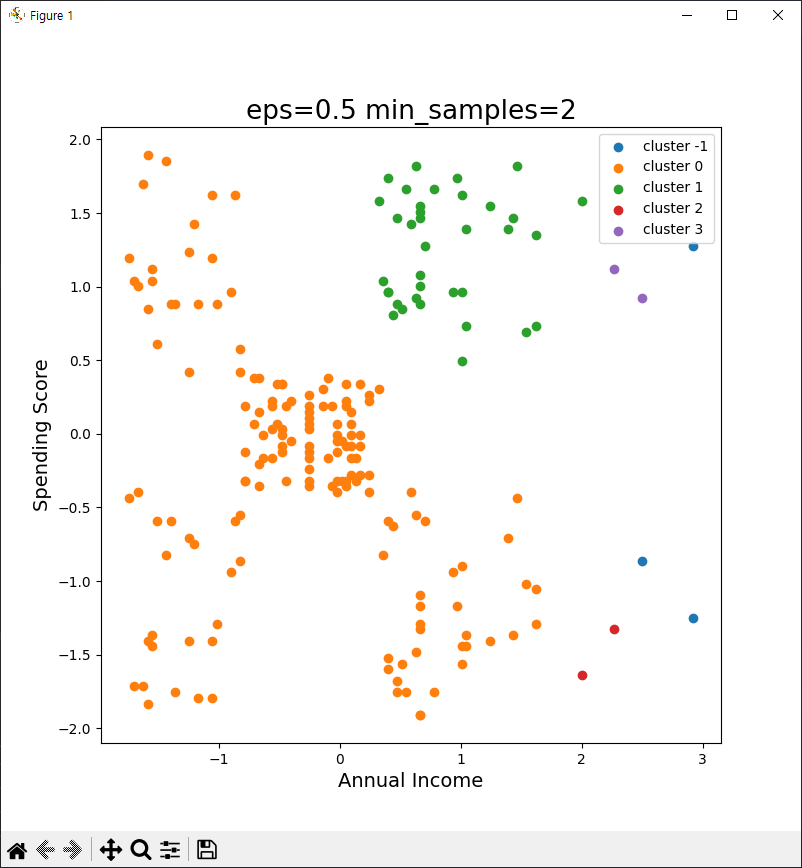
import pandas as pd
import matplotlib.pyplot as plt

from day4.clusteringEx7 import cluster

frame = pd.read_csv('Mall_Customers.csv')
frame.info()

from sklearn.preprocessing import StandardScaler

data = frame[['Annual Income (k$)','Spending Score (1-100)']]

scaler = StandardScaler()
df_scale = pd.DataFrame(scaler.fit_transform(data), columns=data.columns)

from sklearn.cluster import DBSCAN

model = DBSCAN(eps=0.5, min_samples=2)
model.fit(df_scale)
df_scale['cluster'] = model.fit_predict(df_scale)
print(df_scale)

plt.figure(figsize=(8,8))
for i in range(-1, df_scale['cluster'].max() + 1):
    plt.scatter(df_scale.loc[df_scale['cluster'] == i, 'Annual Income (k$)'],
                df_scale.loc[df_scale['cluster'] == i, 'Spending Score (1-100)'],
                label=f'cluster {i}')
plt.legend(loc='best')
plt.title('eps=0.5 min_samples=2', fontsize=19)
plt.xlabel('Annual Income', fontsize=14)
plt.ylabel('Spending Score', fontsize=14)
plt.show()

+AI to AI+