Today

강의

R프로그램 시즌 2 4강

결과

스터디 내용

4. 선형모델 해석, residuals, r squared

year <- c(2000, 2001, 2002, 2003, 2004, 2005, 2006)
value <- c(2.3, 3.2, 4.6, 5.4, 5.8, 6, 6.4)
plot(year, value)

fit <- lm(value ~ year)
abline(fit, col = "red")

fit$coefficients[[2]] # value = 0.92year - 1837.38

fit$residuals # 잔차값

summary(fit)

par(mfrow = c(1,1))
plot(fit)


y = c(1,2,3,4,5,7,8,9,10)
x = c(2,1,4,3,6,5,8,7,9)

plot(x, y)
fit <- lm(y ~ x)
abline(fit , col = "red")
summary(fit)

par(mfrow = c(1,1))
plot(fit)


y = c(1,2,3,4,5,7,8,9,10)
x = c(2,3,4,5,6,2,3,4,5)
fit <- lm(y~x)
abline(fit, col = "red")

plot(fit)

data(iris)
head(iris)

length = iris[which(iris$Species == "setosa"),]$Sepal.Length
width = iris[which(iris$Species == "setosa"),]$Sepal.Width
plot(jitter(length), width, col = "green")
fit2 <- lm(width ~ length)
abline(fit2, col = "yellow")
plot(fit)

par(mfrow=c(1,1))
boxplot(width)

length_new = length[-42]
width_new = width[-42]
boxplot(length_new)
plot(jitter(length_new), width_new, col = "green")

fit <- lm(width_new ~ length_new)
abline(fit, col = 'red')


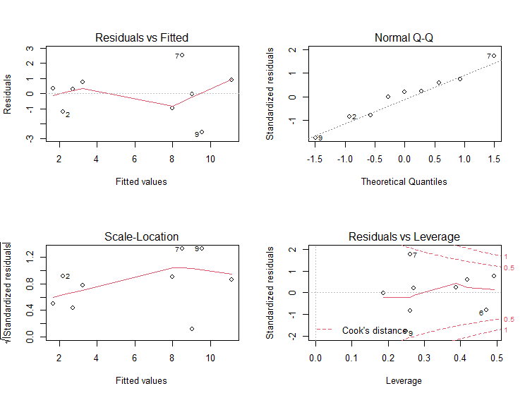
y = c(1,2,3,4,12,7,8,9,10)
z = c(2,1,3,4,12,7,11,9,7)
x = c(2,3,4,5,6,2,3,4,5)
fit <- lm(z ~ x + y)
abline(fit, col = "red")
par(mfrow=c(2,2))
plot(fit)
summary(fit)

Tomorrow

• adsp 3일치, R 5강 실습

Summary

• summary 통계값과 plot 에서 나타나는 네 개의 그래프 해석 방법을 배웠다.