A NEURAL FRAMEWORK FOR GENERALIZED CAUSAL SENSITIVITY ANALYSIS

A NEURAL FRAMEWORK FOR GENERALIZED CAUSAL Sensitivity Analysis

from ICLR2024

Introduce

Causal Sensitivity analysis is that how a cause A affects outcome Y. For example, relationship between the number of times you smoked and the incidence of lung cancer. We can easily think person who smoked many times have higher probability of getting lung cancer. But there is an unobserved confounders like genetic factors.
For example, person who smoked many time has non-cancer gene, person who smoked a few time has a family history of cancer, in this case right one has more probablity than left one.

Existing sensitivity analysis studies are following 3 parts
(1) Category of sensitivity models(like MSM, f-sensitivity model, Rosenbaum's sensitivity model)
(2) treatment type(binary or continuous)
(3) causal query of interest(Expectations, probabilities, and quantiles)

Now, almost of works cannot cover this three things, some research covers (2),(3) only run on MSM.
So this paper introduce follow thing
1 - Define a general class of sensitivity models(a.k.a GTSMs)
2 - Novel neural framework for causal sensitivity analysis NEURALCSA
3 - Provide theoretical base that NEURALCSA learns valid bounds on causal query of interest

Background

Partial identification : Unable to identify point(value of query) because of unobserved confounds, identify under and upper bounds contains target value

Causal Sensitivity analysis : Assume unobserved confounds under sensitivity model, treat partial identification of causal query

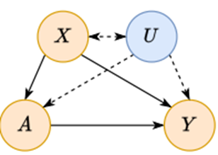
Notations :
X - observed confounds
U - unobserved confounds
A - treatment(similar to constraints)
Y - result

For example, we want to know how exercise(=treatment,A) affects on Cholesterol(causal query). Easily think, people who have many exercising time(=X) have lower Cholesterol(X->Y relation), but there is unobserved confounds like age(unobserved confounds, U).
People who have many age - a health-conscious age- have more exercising time than young people. Old people can have more Cholesterol than young people. In this case, relation (U->Y) isn't controlled. So we will have strange result.
The purpose is disconnecting relation U->Y, than we can get X->Y effects.

fig 1 causal graph :

causal query formulation : $Q(x,a,P)=F(P(Y(a)∣x)$
$F$ is probability to real number matching function
$Q$ about x,a,P means in distribution P, we want effect about x,a -> Y
same as $F(P(Y(a)∣x)$(Intutively, allow treatment a, and set known condition x, get probability about that condition)

But in $P$, there is unobserved confounds, we can only know $P_{obs}$(observed distribution)

They define $P_{obs}$ induced by distribution(X,Y,A,Y) as sensitivity model

Assumption 1
(i) A = a implies Y (a) = Y (consistency);
(ii) P(a | x) > 0 (positivity);
and (iii) Y (a) ⊥⊥ A | X, U (latent unconfoundness).

Task: Given a sensitivity model $M$ and an observational distribution $P_{obs}$, the aim of causal sensitivity analysis is to solve the partial identification problem.

$Q^+_M(x, a) = \displaystyle\sup_{P∈M} Q(x, a, P)$ and $Q^-_M(x, a) = \displaystyle\inf_{ P∈M} Q(x, a, P)$
sup means supremum, inf means infimum

By its definition, the interval
$[Q^-_ M(x, a), Q^+_M (x, a)]$ is the tightest interval that is guaranteed to
contain the ground-truth causal query Q(x, a, P) while satisfying the sensitivity constraints

There is sensitivity parameter $Γ$ which means setting uncertainty(larger $Γ$ means more uncertainty)

They define several sensitivity model like MSM, f-, Rosenbaum as GTSM.
GTSM is formulated as
$P_{obs}(y|x,a) = \int_{}P(y|x,u,a)$$P(u|x,a)$ $du$ (2)

When intervening on the treatment, remove $U-A$ edge in the corresponding causal graph(disconnectiong dependence).
Under assumption 1, that formular is described as
$P(Y (a) = y | x)$ = $\int P(Y(a) = y | x,u)P(u|x)du$ = $\int P(y|x,u,a)$$P(u|x)$ $du$ (3)

**
Sensitivity model M =$\int P(x,u,a,y)du=P_{obs}(x,a,y)$
divide $P(x,a)$,
$P_{obs}(x,a,y) / p(x,a) =\int P(x,u,a,y)du/p(x,a)$
$P_{obs}(y|x,a)=\int P(y|x,u,a)$$P(u|x,a)du$

Under assumption 1,
$P(Y (a) = y | x) / P(x) = \int P(Y (a) = y)/P(x,u) * P(x,u) / P(x) =$
$P(y|x,u,a)$$P(u|x)$ $du$
**

Result we want is distribution affected by A without unobserved confound.
So the goal is disconnecting $U - A$

See (2) and (3), there is only difference on Red and Orange part
$P(u|x,a)$
$P(u|x)$

Before allowing treatment, we have to disconnect $U-A$
Move (2) to (3) means disconnect dependency about A.
So neural model finding sensitivity learns about (2) to (3)

Methodology

NEURALCSA Architecture

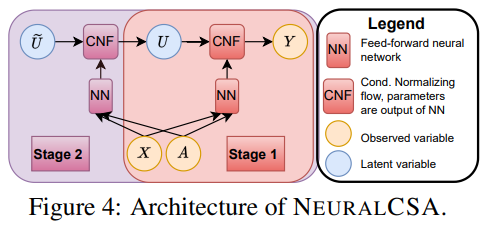
Figure 2

The main objective function concept is training "maximizing red-colored arrows"

$f^*_{x,a}$ means an invertible function $U$->$Y$

They methodology has two procedure.

First is left one, it means input fixed distribution $P^*(U|x,a)$, output $U - A$ independence distribution $P(U|X)$

Second is right one, it means shifting observed and conditioned distribution $P_{obs}(Y|x,a)$ to full and $a$ intervented distribution $P(Y(a)|x)$

Stage 1 neural model $f_{g\theta}^*$, $f^*$ is normalizing flow(distribution to distribution function)

$g\theta$ is fully connected network

optimizing Stage 1 as below loss function

$L_1(θ) = \sum^n_{i=1} log P(f^*_{{g^*_{\theta}} (x_i,a_i)} (U) = yi)$

Intutively understanding,
standard Gaussian distribution U, CNF function $f^*_g$

Input U and output distribution $\hat{y}$, ground truth distribution $y_i$

When $\hat{y}$ and $y_i$ getting different, the loss become smaller.

It seems like training model to "How much different from U-A dependence distribution and U-A independece distribution"

Stage 2
using optimized $\theta$ from Stage 1, goal is optimizing $\eta$

second function $\tilde{f} :\tilde{U} -> \mathcal{U}$

standard distribution $\tilde{U}$ to latent space $\mathcal{U}$

It means parameter described $\eta$ mimics the shift due to unobserved confouning when intervening instead of conditioning
: $P_{obs}(Y | x,a) -> P(Y(a)|x)$

• how they are different? left one means when given a and x, conditional probability $Y$
  right one means set condition a by force, than probability of $Y$

This is considered same as "varing new distribution after intervening from original distribution"

the loss function is following

It is non-trackable function, so we can estimate $L_2$ loss as following:

Here the $\tilde f$ means $\eta$ parameterized model.

$log(P(\tilde{f_\eta^{-1}}(u) = \tilde U )$
It is same as log-likelihood before used.
$\eta^{-1}(u)$ means $U -> \tilde U$
Intuitively, first latent distribution $\tilde U$ and second distribution $U$ are different, loss will down.

It describes that model makes various intervened distribution.

Result and Discussion

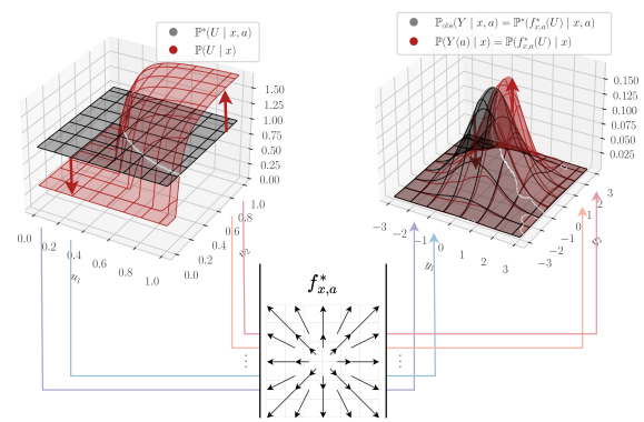
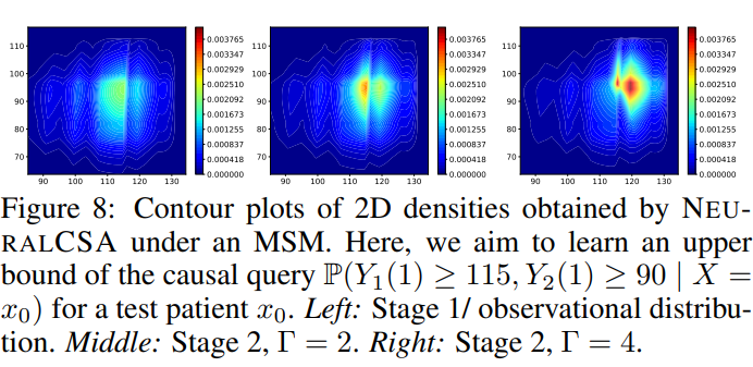
Once NEURALSCA trainied, it can compute not only bounds of causal query, but also shifted distribution by intervening

Experments using synthetic, semi-synthetic, real data.

In synthetic data for MSM,
Validating correctness of NEURALCSA comparing with existing optimal work(closed-form solution for MSM)

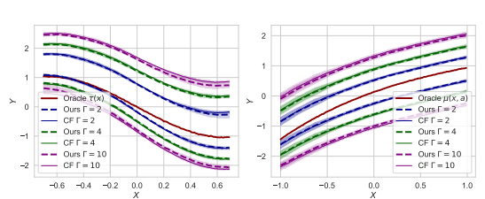
There is no difference about traditional method and neural method.

Using semi-synthetic data for various GTSMs,

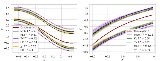
All of GTSMs have in-bound ground truth(Oragle $\tau(x)$)

In real data,
using MSM and making a difference in the sensitivity parameter, result is following

sensitivity parameter is getting bigger, confusion is getting worse.

In this result, NEURALSCA can support any GSTMs certainly, the performance is almost same is traditional optimal method.

Conclusion

In methodological view, NEURALCSA provide new idea for causal sensitivity analysis and partial identification.
Different from traditional method, NEURALCSA learns latent distribution shift when intervening explicitly.
In applied view, NEURALSCA enables practitioners to perform causal sensitivity analysis in numerous settings. Furthermore, it allows for choosing from a wide variety of sensitivity models. It is effective when there is no or less domain knowledge about data-generating process

Own review

First of all, It is very difficult topic.
There are many fomulas, which are not friendly to me.
In addition, I don't domain knowledge about causal sensitivity analysis. Most of deep learning works treat CV,NLP, or unstructured data.
But this is unusuall task.
This paper deals with the distribution to distribution transformation. The goal of this work is almost same performance with existing SOTA, collect various fragments of causal sensitivity analysis that are not organized in traffic.

This approach changes the problem definition P(u ∣ x,a) to create P(u ∣ x), which is a deep learning modeling of the unobserved variable U breaking the relationship of the observed treatment A.
From the perspective of supervised learning, it can be said that this STAGE 1 aims to learn how to break the U-A relationship using known data and generalize it. It is very intuitive to understand.
The purpose of STAGE 2 is very difficult, but if you understand intuitively, it will be an operation to create a distribution to which model report treatment is applied (a distribution to which A is applied, but at this time, it must be an independent distribution for U, so a wide variety of results must be produced).
Almost of deep learning works say "saving time or memory saving or performance improvement applying their own method"
In contrast, this work introduce new and novel method on causal sensitivity analysis. It is meaningful way because of method integration.

Reference

https://assaeunji.github.io/statistics/2020-06-21-matching/
Hitchcock, C. Conditioning, intervening, and decision. Synthese 193, 1157–1176 (2016). https://doi.org/10.1007/s11229-015-0710-8
Hitchcock, Christopher. “Conditioning, Intervening, and Decision.” Synthese, vol. 193, no. 4, 2016, pp. 1157–76. JSTOR, http://www.jstor.org/stable/24704839. Accessed 3 Apr. 2024.