2026.01.22

데이터 분석 도구: Pandas

Pandas 개요

공식문서링크: pandas documentation

NumPy가 숫자 배열을 다루는 데 특화되어 있다면, Pandas는 우리가 흔히 쓰는 엑셀 (table)형태의 데이터를 다루는 데 최적화된 라이브러리 도구이다.

Pandas 설치 및 설정

• pandas 설치
  - pandas를 설치하는 가장 간단한 방법은 pip 명령어를 사용하는 것이다. 터미널이나 커맨드 라인에서 다음 명령어를 입력하면 설치된다.

pip install pandas

conda 사용 시, 다음 명령어로 설치 가능

conda install pandas

환경 설정

• 파이썬 스크립트나 주피터노트북에서 pandas 사용하는 방법:
  여기서 pd는 pandas의 별칭으로 자주 사용되며, 코드의 가독성을 높여준다.

import pandas as pd

• 버전 확인

print(pd.__version__)

다른 라이브러리와 비교 (NumPy, SQL, Excel)

• pandas와 NumPy
  • NumPy는 수치 계산을 위한 배열 기반의 라이브러리이고, pandas는 이를 기반으로 더 복잡한 데이터 구조를 다룬다.
  • pandas는 NumPy 배열을 내부적으로 사용하여 더 효율적으로 대규모 데이터를 처리하지만, 데이터 조작이나 분석에 있어 더 높은 수준의 기능을 제공한다.
• pandas와 SQL
  • SQL은 데이터베이스에서 데이터를 다루는 언어이며, pandas는 로컬 환경에서 데이터를 다룬다.
  • pandas의 DataFrame은 SQL의 테이블과 유사하며, pandas에서는 SQL에서 하는 연산들(선택, 필터링, 조인 등)을 쉽게 수행할 수 있다.
• pandas와 Excel
  • Excel은 GUI 기반의 스프레드시트 소프트웨어로 데이터 분석에 널리 사용되지만, 대규모 데이터 처리나 자동화에는 한계가 있다.
  • pandas는 Excel에서 할 수 있는 대부분의 기능을 코드로 구현할 수 있으며, 특히 데이터의 크기가 커지면 pandas가 훨씬 효율적이다.

---

Pandas의 데이터 구조

pandas는 Series와 DataFrame 이라고 하는 두가지 주요 데이터 구조를 제공함

• Series: 1차원 배열로, 인덱스를 포함하며 데이터를 저장한다. (데이터에 고유한 인덱스를 부여하여 데이터에 접근할 수 있다.)
• DataFrame: 2차원 테이블 형식의 데이터 구조로 여러 개의 Series가 모여 테이블을 이루며, 각 컬럼은 동일한 인덱스를 공유한다. (행과 열 모두 인덱스를 통해 접근할 수 있다.)

(1) Series:

Series: 1차원 데이터
엑셀 시트에서 열(column)하나를 떼어낸 것과 같은 형태로, 데이터값(value) 뿐만 아니라 각 값에 이름을 붙인 인덱스(index)가 항상 쌍으로 존재한다.
구조: index + data values

NumPy의 1차원 배열과 유사하며 인덱스와 데이터를 함께 저장
데이터는 숫자, 문자열, 불리언, 또는 다른 데이터 타입을 포함할 수 있음

• index(label)을 통해 조작/처리 가능한 1차원 배열
• 엑셀의 열(column) 하나라고 생각하면 쉬워
• 데이터(value)와 각 데이터에 대응하는 인덱스(index)가 한 쌍으로 묶여있어
• 별도로 인덱스를 지정하지 않았기 때문에 0, 1, 2, 3, 4라는 기본 정수형 인덱스가 자동으로 부여돼

생성방법
pd.Series()함수 사용하여 생성

import pandas as pd

# 리스트로 Series 생성
s = pd.Series([10, 20, 30, 40], index=['a', 'b', 'c', 'd'])
print(s)

특징

• 각 데이터는 고유한 인덱스를 가지며, 이를 통해 데이터에 쉽게 접근할 수 있음
• dtype은 Series 내부의 데이터 타입을 나타냄

데이터 선택
Series의 각 값은 인덱스를 이용해 선택할 수 있음

# 인덱스를 이용한 선택
print(s['b'])  # 20

# python list 활용
stocks_ser = pd.Series(['NVDA', 'MSFT', 'AAPL', 'GOOG', 'TSLA'])
# 속성 설정: 
stocks_ser.name = '미국 주식' # name 속성 (인스턴스)
#전체 데이터 출력: 
print(stocks_ser)           # 데이터, row index, Name, dtype
# 결과값:
# 왼쪽(0~4): 행 번호인 index
# 오른쪽(NVDA~TSLA): 실제 data
# Name: 위에서 설정한 시리즈의 이름
# dtype: 데이터의 타입. 문자열 데이터는 판다스에서 보통 object로 표시

# 특정 데이터 접근 (indexing)
print(stocks_ser[3])  # GOOG / 리스트와 마찬가지로 대괄호 [ ] 를 사용해서 특정위치의 데이터를 가지고 와.
# 자료형 확인: 이 변수가 일반 파이썬 리스트가 아니라, 판다스의 시리즈 객체임을 증명
print(type(stocks_ser))

# NumPy ndarray 활용
nums_ser = pd.Series(np.random.randn(5), index=['a', 'b', 'c', 'd', 'e'])  
                                       # Series 생성 시 index label 지정 가능
print(nums_ser)       # Series 전체 출력 

# print(nums_ser[4]) -> ver.2.x.x (o) -> ver.3.0.0 (x)
# ver.2.x.x (index 숫자로 가능) -> ver.3.0.0 (index label이 설정된 경우 불가)
# eg)
# loc: 내눈에 보이는 이름(label)표를 보고 찾는다
#iloc: 컴퓨터가 관리하는 순서(position) 번호를 보고 찾는다.

print(nums_ser['e'])   # -> 결과값: 인덱스 'e'에 해당하는 난수값 출력
# loc (label-based): 라벨 이름을 사용한 접근 -> 결과는 위와 동일. 명시적으로 '라벨'을 쓰겠다고 선언하는 방식
print(nums_ser.loc['e']) #.찍고 loc[] 오면 이것은 속성 / loc(location): 인덱스라벨을 통한 참조
# 위치 번호 (0부터 시작)을 사용한 접근 -> 결과: 5번째 (인덱스4)값인 'e'의 위치 값을 출력
print(nums_ser.iloc[4])  # iloc(integer location): 인덱스를 통한 참조

# python dictionary 활용 (key가 index label, value가 값이 됨)
info = {
    'a': 100,
    'b': 200,
    'c': 300
}
info_ser = pd.Series(info)
print(info_ser)

info_ser.index = ['A', 'B', 'C']
print(info_ser)

# scalar value 활용
num_ser = pd.Series(5.5)
num_ser = pd.Series(5.5, index=['ㄱ', 'ㄴ', 'ㄷ', 'ㄹ', 'ㅁ'])
print(num_ser)

Series 속성

movies = ['만약에 우리', '프로젝트 Y', '신의 악단', '아바타: 불과 재', '천공의 성 라퓨타']
movies_ser = pd.Series(movies)
movies_ser

출력값:
0       만약에 우리
1       프로젝트 Y
2        신의 악단
3    아바타: 불과 재
4    천공의 성 라퓨타
dtype: str

# 값으로만 이루어진 ndarray 반환
print(movies_ser.to_numpy())       # ['만약에 우리' '프로젝트 Y' '신의 악단' '아바타: 불과 재' '천공의 성 라퓨타']
print(type(movies_ser.to_numpy()))  # <class 'numpy.ndarray'>

# [참고] value 속성은 2.x.x 버전에서는 to_numpy()와 같은 기능을 했으나 3.0.0 ver.에서는 array와 같은 기능을 하며 사용 지양함.
# print(movies_ser.values)
# print(type(movies_ser.values))

# pandas의 확장 Array 객체로 값 반환
print(movies_ser.array)
print(type(movies_ser.array))

# <StringArray>
# ['만약에 우리', '프로젝트 Y', '신의 악단', '아바타: 불과 재', '천공의 성 라퓨타']
# Length: 5, dtype: str
# <class 'pandas.arrays.StringArray'>

# index를 별도 지정하지 않은 경우 기본적으로 숫자 인덱스 (RangeIndex)
print(movies_ser.index)   # RangeIndex(start=0, stop=5, step=1)

# 라벨을 지정한 경우 라벨 인덱스 
movies_ser.index = ['1st', '2nd', '3rd', '4th', '5th']
print(movies_ser.index)   # Index(['1st', '2nd', '3rd', '4th', '5th'], dtype='str')

print(movies_ser.dtype) # 자료타입               # str
print(movies_ser.shape) # 구조 (형태)            # (5,)
print(movies_ser.ndim)  # 차원 (깊이)            # 1
print(movies_ser.size)  # 크기 (요소 개수)        # 5

# is_unique: 시리즈가 가진 값이 모두 고유한 값인지의 여부 (True: 중복값 X / False: 중복값 O)

movies_ser.is_unique             # True

Series 메서드

nums_ser = pd.Series([2026, 1, 22, 11, 23])

# 값 연산
print(nums_ser.sum())      # 총합 (누적 합)    -> 2083
print(nums_ser.mean())     # 평균				-> 416.6
print(nums_ser.product())  # 누적 곱 		   -> 11276716

# 데이터 확인
print(nums_ser.head(2))    # 앞에서부터 일부 데이터를 조회 (기본값=5)
print(nums_ser.tail(3))    # 뒤에서부터 일부 데이터를 조회 (기본값=5)

# Series 메타데이터 (meta data): not-null 여부 확인, 자료형 확인,...
nums_ser.info()

# Series의 데이터를 분석/설명
nums_ser.describe()

movies_ser.describe()
# 데이터의 type에 따라 describe()결과 달라질 수 있음

S&P 500 데이터 활용

pd.read_csv('./data/S_P500_Prices.csv')

# read_csv(file_path): file_path 파일을 읽어와 DataFrame 형태로 반환
sp_500 = pd.read_csv('./data/S_P500_Prices.csv')
type(sp_500)        # pandas.DataFrame

# df.squeeze(): DataFrame 의 Series가 하나인 경우 Series 객체 반환
sp_500_ser = sp_500.squeeze()
type(sp_500_ser)    # pandas.Series

# sp_500_ser의 메타 데이터 확인
sp_500_ser.info()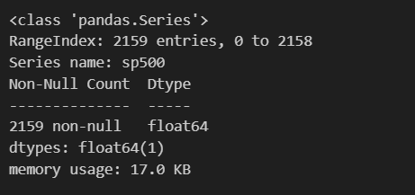

# sp_500_ser의 데이터 요약 확인
sp_500_ser.describe()

# sp_500_ser의 형태, 요소 개수, 차원수 확인
sp_500_ser.shape, sp_500_ser.size, sp_500_ser.ndim

# sp_500_ser의 요소개수, 최소값, 중위값, 최대값, 평균값, 표준편차값, 분산값 각각 출력
sp_500_ser.count(), sp_500_ser.min(), sp_500_ser.median(), sp_500_ser.max(), sp_500_ser.mean(), sp_500_ser.std(), sp_500_ser.var()

indexing & slicing

# [indexing] 인덱스 50의 값 가져오기
print(sp_500_ser[50])
print(sp_500_ser.iloc[50])

# [slicing] 인덱스 100~200 값 가져오기
print(sp_500_ser[100:201])
print(sp_500_ser.iloc[100:201])

# [fancy indexing] 인덱스 1000,2000의 값 동시에 가져오기
# indices = [1000, 2000]
print(sp_500_ser[[1000, 2000]])
# or
print(sp_500_ser.iloc[[1000, 2000]])

# [boolean indexing] 데이터 값이 3000 이상인 값 가져오기
print(sp_500_ser[sp_500_ser >= 3000])

값 존재 여부 판단

print(3333.689941 in sp_500_ser)   # 라벨 중에 3333.689941 이 있니?
print(3333.689941 in sp_500_ser.to_numpy()) # 갖고 있는 값 중에 3333.689941이 있니?

print(sp_500_ser.isin([3333.689941]).any())
# False
# True
# True

# isin(): 각 값에 대해 일치하는지 판단해 bool series 반환
bool_series = sp_500_ser.isin([3333.689941])

# any(): True가 하나라도 존재하면 True
bool_series.any()

print(sp_500_ser.sort_values()) # 정렬된 Series 객체 반환
print(sp_500_ser)             # 원본 Series 에 영향 없음

sp_500_ser.sort_values(ascending=False) # 내림차순 정렬
print(sp_500_ser)

sp_500_ser.sort_values(inplace=True)    
# 원본을 수정하는 inplace 연산 (sp_500_ser = sp_500_ser.sort_values() 와 같은 결과)
print(sp_500_ser)

(2) DataFrame

DataFrame은 행(row)과 열(column)로 이루어진 2차원 데이터 구조로, 다양한 데이터 타입을 포함할 수 있다. DataFrame은 엑셀 시트나 SQL 테이블과 유사한 구조를 가지고 있다.

• Series를 묶어낸 자료형으로 2차원 배열(=행렬, 표)
• 인덱스 라벨을 기준으로 데이터를 자동으로 정렬

생성 방법
DataFrame은 다양한 방법으로 생성할 수 있다. 대표적인 방법으로는 딕셔너리 또는 리스트를 사용하는 방법이 있다.

data = {
    'Name': ['Alice', 'Bob', 'Charlie', 'David'],
    'Age': [25, 30, 35, 40],
    'City': ['New York', 'Los Angeles', 'Chicago', 'Houston']
}

df = pd.DataFrame(data)
print(df)

특징

• 각 열(Column)은 고유한 Series로 간주된다.
• 행과 열에는 각각의 인덱스와 컬럼 라벨이 있어 데이터를 쉽게 선택할 수 있다.

데이터 선택

• DataFrame에서 특정 열을 선택하려면 열 이름을 사용하면 된다.

# 특정 열 선택
print(df['Name'])

• 행을 선택하려면 loc나 iloc을 사용할 수 있다.

# 특정 행 선택 (인덱스 기준)
print(df.loc[1])  # 두 번째 행 선택

Series와 DataFrame의 차이점

• Series는 1차원 데이터 구조로, 데이터에 고유한 인덱스를 부여하여 데이터에 접근할 수 있다.
• DataFrame은 2차원 데이터 구조로, 여러 개의 Series가 모여 테이블을 이루며, 행과 열 모두 인덱스를 통해 접근할 수 있다.

DataFrame 생성

# python dictionary-list 활용: 딕셔너리의 Key가 열(column) 이름이 되고, Value(리스트)가 데이터
data = {
    'one': [1, 2, 3, 4, 5],
    'two': ['가', '나', '다', '라', '마'],
    'three': [1.23, 2.34, 3.45, 4.56, 5.67],
    'four': True   # 모든 list 요소의 length를 맞춰야 하지만, scalar value 는 예외
}
df = pd.DataFrame(data)
df

# python list-dictionary 활용
data = [
    {'a': 1, 'b': 2, 'c': 3},
    {'b': 5, 'c': 6},             # 'a' == NaN (Not a Number)
    {'a': 7, 'b': 8, 'c': 9}
]
df = pd.DataFrame(data)
df

FYI - Numpy로 데이터를 생성하고, 이를 활용해 Pandas DataFrame을 만든 뒤 속성을 변경하는 과정

# NumPy 2차원 ndarray 활용
arr = np.random.randn(2, 3)
# NumPy의 randn은 소수점이 있는 실수형 데이터를 생성하므로, 이 데이터프레임의 모든 값의 타입은 float64가 됨

# DataFrame 생성 시 index, columns 속성 지정 가능 (행과 열 이름 지정)
df = pd.DataFrame(arr, index=['가', '나'], columns=['A', 'B', 'C'])

# 속성(Attribute) 접근 및 수정: DataFrame 속성으로 접근해 수정 가능
df.index = ['1번학생', '2번학생']
df.columns = ['귀여움', '사랑스러움', '간지']
df

data = {
    '이름': ['다람쥐', '원숭이', '호랑이'],
    '위치': ['독산', '서초', '안양'],
    '성별': ['F', 'M', 'M']
}
teacher_df = pd.DataFrame(data)
# teacher_df = pd.DataFrame(data, index=['Squirrel', 'Monkey', 'Tiger'])
teacher_df

# 전치행렬
teacher_df.T

DataFrame 속성

print(teacher_df.index)    # row(행) 식별 --- RangeIndex(기본숫자), Index(label)
print(teacher_df.columns)  # column (열) 식별 --- Index(label), [RangeIndex(기본숫자, 전치가 일어난 경우...)]

print(teacher_df.T)

print(teacher_df.shape)  # 구조 (형태)
print(teacher_df.size)   # 요소 개수
print(teacher_df.ndim)   # 차원 (깊이)
print(teacher_df.dtypes)  # 요소의 자료형 (컬럼별 자료형)

print(teacher_df.values)      # DataFrame 이 가진 값만 추출
print(type(teacher_df.values))

DataFrame 메서드

bank_client_df = pd.DataFrame({
    'Client ID': [1, 2, 3, 4],
    'Client Name': ['Ali', 'Steve', 'Nicole', 'Morris'],
    'Net worth [$]': [35000, 3000, 100000, 2000],
    'Years with bank': [4, 7, 10, 15]
})
bank_client_df

데이터 확인

print(bank_client_df.head(2)) # 상위 2개의 행을 보여줘 / 데이터가 밀리지 않고 컬럼명에 맞게 잘 들어갔는지 확인할 때 쓸수있음
print(bank_client_df.tail(1)) # 가장 마지막 1개의 행을 보여줘 / 전체 데이터가 총 몇 번 인덱스까지 있는지, 끝부분에 결함은 없는지 확인할 때 쓸수있음

bank_client_df.info() # 데이터의 골격 (기술적인 상태)확인

# RangeIndex: 전체 행의 개수 (4 entries, 0 to 3)를 보여줍니다.
# Data columns: 총 컬럼 개수와 각 컬럼의 이름을 나열합니다.
# Non-Null Count: 빈 값(결측치)이 아닌 데이터가 몇 개인지 보여줍니다. (여기서는 모두 4개이므로 빈 값이 없음을 알 수 있습니다.)
# Dtype: 데이터 타입을 보여줍니다.
# int64: 정수 (ID, 자산, 기간)
# object: 문자열 (이름)
# Memory Usage: 이 표가 메모리를 얼마나 차지하는지 보여줍니다.

bank_client_df.describe() # 통계요약표 - 숫자형 데이터에 대해서만 기본적인 통계치를 계산해줌

# count	데이터 개수
# mean	평균값
# std	표준편차 (데이터가 평균에서 얼마나 떨어져 있는지)
# min	최솟값
# 25%	하위 25% 지점의 값 (1사분위수)
# 50%	중앙값 (2사분위수)
# 75%	상위 25% 지점의 값 (3사분위수)
# max	최댓값

Indexing & Slicing

• iloc: 행(row), 열(column) 순으로 탐색
• loc: 행(row), 열(column) 순으로 탐색
• iloc나 loc를 쓰지 않고 대괄호를 붙여 사용하면 df[컬럼명]을 넣는 식

1. iloc (integer location)

# indexing: 특정 행을 Series로 반환

print(bank_client_df.iloc[0])
print(type(bank_client_df.iloc[0]))
print(bank_client_df.iloc[0].index)
print(bank_client_df.iloc[0].name)

# slicing: 해당되는 행을 DataFrame 으로 반환
print(type(bank_client_df.iloc[:2]))
bank_client_df.iloc[:2]

# fancy indexing: 해당되는 행을 DataFrame으로 반환
print(type(bank_client_df.iloc[[0, 1]]))  #fancy indexing
bank_client_df.iloc[[0, 1]]

# fancy indexing 을 통한 조회는 결과가 1개여도 DataFrame 타입으로 반환 (차원 유지)
# 일반적인 indexing(e.g) bank_client_df.iloc[0]은 Series 타입으로 반환 (차원 제거)
print(type(bank_client_df.iloc[[0]]))
bank_client_df.iloc[[0]]   

# 2차원 indexing : 특정 행, 특정 열의 값 반환
bank_client_df.iloc[0, 1]    # iloc[행 index, 열 index]

# 2차원 slicing: 해당되는 행, 해당되는 열의 데이터 DataFrame으로 반환
print(type(bank_client_df.iloc[:2, 2:]))   # 슬라이싱(:) 을 쓰면 DataFrame(2차원) 유지
bank_client_df.iloc[:2, 2:]                # 0~1번 행(2개)를 가져오고 열은 2번 열부터 끝까지 가져와

# 2차원 indexing + slicing: 해당되는 데이터를 Series로 반환
print(type(bank_client_df.iloc[:2, 1]))   # 특정 인덱스 번호를 직접 쓰면 Series(1차원) 으로 차원 축소됨
bank_client_df.iloc[:2, 1]              # 0~1번 행(2개)를 가져오되, 열은 딱 1번열(client name)하나만 지정해서 가져와

# 만약 열이 하나라도 DataFrame 형태를 유지하고 싶다면 범위 형태(1:2)를 쓰거나 리스트형태([1])을 쓰면 됨.
df_output = bank_client_df.iloc[:2, [1]] 
print(type(df_output))

2. loc (location)

# loc 사용하기 위해 index 에 label 설정
bank_client_df.index = ['c1', 'c2', 'c3', 'c4']
bank_client_df

# loc => location -> index label

# 1. c3의 데이터 조회
#  indexing: 특정 행을 Series로 반환
print(type(bank_client_df.loc['c3']))
bank_client_df.loc['c3']

# 2. c2 ~ c4의 데이터를 2명씩 건너뛰며 조회
#  slicing: 해당되는 행을 DataFrame으로 반환
print(type(bank_client_df.loc['c2':'c4':2]))
bank_client_df.loc['c2':'c4':2]

# 3. 2에서 조회한 데이터의 Client name만 조회
#  2차원 indexing + slicing: 해당되는 데이터를 Series로 반환
print(type(bank_client_df.loc['c2':'c4':2, 'Client Name']))
bank_client_df.loc['c2':'c4':2, 'Client Name']

# 4. 2에서 조회한 데이터의 Client name 컬럼부터 Net worth [$] 컬럼까지 조회
#  2차원 slicing: 해당되는 행, 해당되는 열의 데이터 DataFrame으로 반환
print(type(bank_client_df.loc['c2':'c4':2, 'Client Name':'Net worth [$]']))
bank_client_df.loc['c2':'c4':2, 'Client Name':'Net worth [$]']

# 5. 2에서 조회한 데이터의 Client name과 Years with bank 컬럼만 조회
#  fancy indexing: 해당되는 데이터를 DataFrame으로 반환
print(type(bank_client_df.loc['c2':'c4':2, ['Client Name', 'Years with bank']] ))
bank_client_df.loc['c2':'c4':2, ['Client Name', 'Years with bank']] 

# 이름이 Steve인 고객 정보 출력
bank_client_df.loc[bank_client_df['Client Name'] =='Steve']

3. loc나 iloc없이 대괄호 [] 접근

# 해당 컬럼에 대한 데이터를 Series로 반환
bank_client_df['Client Name']

# 컬럼명 배열로 fancy indexing 가능
bank_client_df[['Client Name', 'Net worth [$]']]

filter()

bank_client_df.filter(items=['Client Name', 'Net worth [$]'])

bank_client_df.filter(like='$', axis=1)

bank_client_df

bank_client_df.filter(like='4', axis=0)

행 추가 및 삭제