[논문리뷰] Generative Modeling by Estimating Gradients of the Data Distribution (NCSN, 2019)
Diffusion Models
목록 보기
2/8
Introduction : previous Generative model
- likelihood-based model
- log-likelihood를 objective으로 사용
- normalized probability model을 구하기 위해 복잡한 아키텍처가 필요하거나 (autoregressive models, flow models)
- surrogate loss를 써야 하는 단점 (ELBO in autoencoder)
- GAN
- adversarial training이라는 구조적 문제 때문에 unstable
- GAN objective는 모델끼리 비교하기가 까다로움
Score-based generative modeling
- dataset : unknown data distribution 로부터 얻은 i.i.d. samples
- 우리는 궁극적으로 를 알고 싶다!
- likelihood methods에서는 를 계산하는 식으로 접근한다
- idea : log probability density의 gradient를 구하면 기울기를 따라 샘플링할 수 있고, 결국 를 아는 것과 같은 효과를 낼 수 있다!
- score := gradient of log probability density
- score network
- neural network parameterized by
- 우리는 이 score network로 score를 모방하고 싶다
- Goals
- generative models의 목표는 given dataset을 가지고 를 모방한 모델을 학습시키는 것
- two parts of score-based generative modeling
Challenges of score-based generative modeling
The manifold hypothesis
- 문제 상황
- 데이터셋은 high dimensional space (a.k.a. ambient space)에서 정의되지만 실상 low dimensional manifolds에만 집중적으로 분포하는 경우가 많다
- 요 현상이 manifold learning의 기본 아이디어가 됨
- 왜 문제가 되나?
- low dimensional manifold에서는 score가 정의되지 않는다! (데이터가 없으니 기울기도 없음)
- score network와 true score를 matching시키는 score matching objective는 data distribution의 support가 whole space일 때만 consistent한 score를 얻는다
- ResNet, CIFAR-10, sliced score matching으로 실험해봤더니
- 그냥 데이터셋을 쓰면 loss가 잘 안 줄어드는데
- data에 약간의 perturbation을 걸어서 perturbed data distribution이 전체 space를 support로 갖게 만들면 loss가 안정적으로 잘 줄어들었다
Low data density regions
- low density regions에 data가 부족하면
1. score matching에서도 문제를 겪고
2. sampling하기도 어려워진다
Inaccurate score estimation with score matching
- 전체 space 중에 probability density가 거의 0인 구역 이 있다 치면 ()
- 로부터 샘플링한 데이터셋에는 에 속하는 데이터가 아예 없을 확률이 높다
- 그렇게 되면 score matching을 정확하게 해도 구역에서는 score가 정의되지 않거나 부정확하게 구해진다
Slow mixing of Langevin dynamics
- 가 두 개의 distribution의 mixture이고, 두 distribution 사이에는 low density region이 있다 치자
- 여기서 log gradient를 취하면 과 의 score 둘 다 를 날려버린다
- approximately disjoint supports를 가지는 distribution끼리 섞으면 이렇게 됨
- 이 상태로 Langevin dynamics를 진행하면 distribution끼리의 relative weights를 반영하지 못함
Noise Conditional Score Networks (NCSN)
NCSN
- data에 Gaussian perturbation을 가하면 위에서 서술한 문제들을 해결 가능!
1) perturb data using various levels of noise
2) simultaneously estimate scores corresponding to all noise levels by training a single conditional score network
3) use Langevin dynamics to generate samples after training - definition
- Let be a positive geometric sequence that satisfies
- 여기서 은 위에서 서술한 문제를 해결하기에 충분히 큰 noise여야 하고
- 은 true data에 거의 영향을 주지 않을 정도로 작은 noise여야 한다
- Let denote the perturbed data dist.
- 모든 noise level 에 대해 의 score를 예측하는 score network 를 학습시킨다 == Noise Conditional Score Network
- Let be a positive geometric sequence that satisfies
- Model architecture
- 본 논문에서는 image domain만 다룸
- UNet + dilated convolution을 사용
- score matching만 제대로 할 수 있으면 어떤 구조를 써도 ok
Learning NCSN via score matching
- using Denoising score matching, objective is given as
- 우리는 noise distribution을 로 잡았으므로,
- 따라서 score matching objective는 아래와 같이 정리됨
- coefficient
- 얘를 결정하는 방법에는 여러 가지가 있지만, 의 크기가 대충 일정한 게 좋아보임
- 실험적으로, model이 optimal하게 학습되었을 때 는 대략 에 비례했음
- 따라서 로 세팅
- 모든 항이 상수에 비례한다
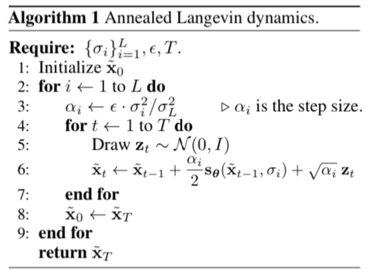
NCSN inference via annealed Langevin Dynamics
- 기존 Langevin dynamics는 fixed step size로 진행됨
- sampling 초반(가 클 때)에는 step size가 크고 점점 줄어들어 마지막에는 이 되도록 조절하는 annealed Langevin Dynamics 도입
-
- signal to noise(SNR) ratio 를 일정하게 유지하기 위해 이렇게 설정함