[w5d5] Histogram Stretch, Filtering

(Ubuntu 18.04.6 LTS)
2022.03.18.
C++, VS code 사용
프로그래머스 자율주행 데브코스 3기

histogram stretch

이전의 대조는 특정값을 기준으로 분포를 나누는 형태로 주어졌다. 그 값은 주로 평균값이나 밝기의 중간값인 128인 경우가 많았다.

dst = src + (src - m) * alpha
dst = src + (128 - m)

histogram stretch는 histogram 상 분포에서 최대,최소값을 이용하여 밝기를 조절한다.

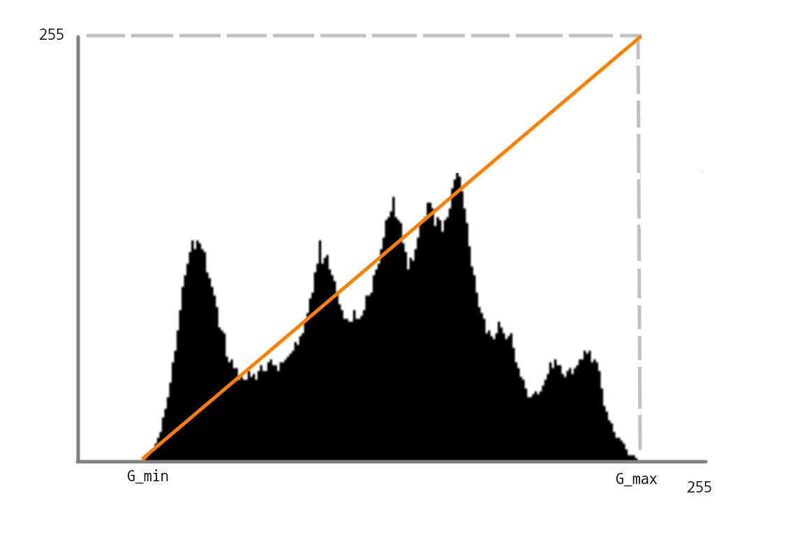
적용되는 공식은 아래와 같다.

dst = 255/(G_max - G_min) * (src - G_min)

openCV에서 최대 최소값을 구하는 함수는 cv::minmaxLoc이다.

void cv::minMaxLoc 	( 	InputArray  	src,
		double *  	minVal,
		double *  	maxVal = 0,
		Point *  	minLoc = 0,
		Point *  	maxLoc = 0,
		InputArray  	mask = noArray() 
	) 		

minVal, maxVal에는 각각의 값을 담을 double형 변수의 주소를 넣으면 된다.
Point도 추가적으로 넣으면 해당 위치를 Point로 받을 수 있다.

cv::normalize를 이용해서도 histogram stretch를 수행할 수 있다.

void cv::normalize 	( 	InputArray  	src,
		InputOutputArray  	dst,
		double  	alpha = 1,
		double  	beta = 0,
		int  	norm_type = NORM_L2,
		int  	dtype = -1,
		InputArray  	mask = noArray() 
	) 		

norm_type을 NORM_MINMAX로 설정한 경우 alpha는 최소, beta는 최대값으로 사용할 수 있다.

// 예시 코드
#include <iostream>
#include "opencv2/opencv.hpp"

int main()
{
    cv::Mat src = cv::imread("./resources/lenna.bmp",cv::IMREAD_COLOR);

    if (src.empty()){
        std::cerr << "Image load failed!" << std::endl;
        return -1;
    }
    double gmin,gmax;
    cv::minMaxLoc(src,&gmin,&gmax);
    cv::Mat dst = (src-gmin)*255/(gmax-gmin);

    cv::Mat dst2,src2;
    cv::cvtColor(src,src2,cv::COLOR_BGR2GRAY);
    cv::normalize(src2,dst2,0,255,cv::NORM_MINMAX);

    cv::imshow("image",src);
    cv::imshow("dst",dst);
    cv::imshow("image2",src2);
    cv::imshow("dst2",dst2);

    cv::waitKey();
    cv::destroyAllWindows();
    return 0;
}

하지만 최대값, 최소값 주변의 pixel 수가 적거나 noise가 발생하였을 때 단순한 최대 최소값만으로는 수행에 어려움이 있다. 일정 비율을 넘었을 때 그 값을 기준으로 histogram stretch를 수행할 수 있으며 그 코드는 아래와 같다.

#include "opencv2/opencv.hpp"
#include <iostream>

void histogram_stretching(const cv::Mat& src, cv::Mat& dst);
void histogram_stretching_mod(const cv::Mat& src, cv::Mat& dst);

int main()
{
	cv::Mat src = cv::imread("./resources/lenna.bmp", cv::IMREAD_GRAYSCALE);

	if (src.empty()) {
		std::cerr << "Image load failed!" << std::endl;
		return -1;
	}

	cv::Mat dst1, dst2;
	histogram_stretching(src, dst1);
	histogram_stretching_mod(src, dst2);

	cv::imshow("src", src);
	cv::imshow("dst1", dst1);
	cv::imshow("dst2", dst2);
	cv::waitKey();
}

void histogram_stretching(const cv::Mat& src, cv::Mat& dst)
{
	double gmin, gmax;
	cv::minMaxLoc(src, &gmin, &gmax);

	dst = (src - gmin) * 255 / (gmax - gmin);
}

void histogram_stretching_mod(const cv::Mat& src, cv::Mat& dst)
{
	int hist[256] = {0,};

	for(int y=0;y<src.rows;y++){
		for(int x=0;x<src.cols;x++){
			hist[src.at<uchar>(cv::Point(y,x))]+=1;
		}
	}

	int gmin, gmax;
	int ratio = int(src.cols * src.rows * 0.01);
	
	for (int i = 0, s = 0; i < 255; i++) {
		s += hist[i];
		if (s>=ratio){
			gmin = i;
			break;
		}
	}

	for (int i = 255, s = 0; i >= 0; i--) {
		s += hist[i];
		if (s>=ratio){
			gmax = i;
			break;
		}
	}

	dst = (src-gmin)/(gmax-gmin)*255;
}

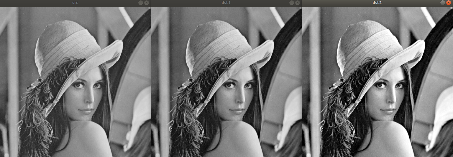
가장 왼쪽이 기존 사진, 두번째가 일반적인 histogram stretch, 3번째 사진이 1%에서 histogram stretch를 한 것으로, 조금 더 선명도가 높은 것을 볼 수 있다.

histogram equalization

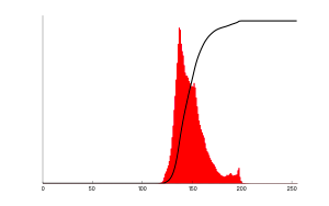
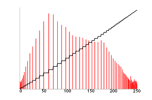
histogram equalization은 전체 구간에서 균일한 분포로 나타나도록 변경하는 기법으로, 히스토그램을 구하고, 정규화한 후 누적 분포 함수를 구한뒤 최대값을 곱한 값을 반올림한다. 아래의 위키 사이트의 내용을 보고 작성하였다.

https://en.wikipedia.org/wiki/Histogram_equalization

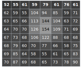
이미지의 명암값들을 텍스트 파일에 넣었다. 이후 파이썬을 이용해서 개수를 구해보았다.

# python 3
f = open("counti.txt",'r')
hist = [0]*256
while True:
    line = f.readline()
    if not line: break
    hist[int(line)]+=1
hist_sum = float(sum(hist))
cdf = 0
for idx, count in enumerate(hist):
    if (count!=0):
        norm_hist=count/hist_sum
        cdf += norm_hist
        dist_val = int(round(cdf*255,0))
        print(f'{idx:3}: count: {count}, norm_hist = {norm_hist:.3f}, cdf = {cdf:.3f}, dst_val = {dist_val}')
f.close

결과값은 아래와 같다. count는 개수, norm_hist는 전체 개수로 나눈 값, cdf는 cumulative distribution function이다. 이를 255 범위에서 평활화하기 위해서는 cdf에 255를 곱한 후 반올림해주었다.

 52: count: 1, norm_hist = 0.016, cdf = 0.016, dst_val = 4
 55: count: 3, norm_hist = 0.047, cdf = 0.062, dst_val = 16
 58: count: 2, norm_hist = 0.031, cdf = 0.094, dst_val = 24
 59: count: 3, norm_hist = 0.047, cdf = 0.141, dst_val = 36
 60: count: 1, norm_hist = 0.016, cdf = 0.156, dst_val = 40
 61: count: 4, norm_hist = 0.062, cdf = 0.219, dst_val = 56
 62: count: 1, norm_hist = 0.016, cdf = 0.234, dst_val = 60
 63: count: 2, norm_hist = 0.031, cdf = 0.266, dst_val = 68
 64: count: 2, norm_hist = 0.031, cdf = 0.297, dst_val = 76
 65: count: 3, norm_hist = 0.047, cdf = 0.344, dst_val = 88
 66: count: 2, norm_hist = 0.031, cdf = 0.375, dst_val = 96
 67: count: 1, norm_hist = 0.016, cdf = 0.391, dst_val = 100
 68: count: 5, norm_hist = 0.078, cdf = 0.469, dst_val = 120
 69: count: 3, norm_hist = 0.047, cdf = 0.516, dst_val = 131
 70: count: 4, norm_hist = 0.062, cdf = 0.578, dst_val = 147
 71: count: 2, norm_hist = 0.031, cdf = 0.609, dst_val = 155
 72: count: 1, norm_hist = 0.016, cdf = 0.625, dst_val = 159
 73: count: 2, norm_hist = 0.031, cdf = 0.656, dst_val = 167
 75: count: 1, norm_hist = 0.016, cdf = 0.672, dst_val = 171
 76: count: 1, norm_hist = 0.016, cdf = 0.688, dst_val = 175
 77: count: 1, norm_hist = 0.016, cdf = 0.703, dst_val = 179
 78: count: 1, norm_hist = 0.016, cdf = 0.719, dst_val = 183
 79: count: 2, norm_hist = 0.031, cdf = 0.750, dst_val = 191
 83: count: 1, norm_hist = 0.016, cdf = 0.766, dst_val = 195
 85: count: 2, norm_hist = 0.031, cdf = 0.797, dst_val = 203
 87: count: 1, norm_hist = 0.016, cdf = 0.812, dst_val = 207
 88: count: 1, norm_hist = 0.016, cdf = 0.828, dst_val = 211
 90: count: 1, norm_hist = 0.016, cdf = 0.844, dst_val = 215
 94: count: 1, norm_hist = 0.016, cdf = 0.859, dst_val = 219
104: count: 2, norm_hist = 0.031, cdf = 0.891, dst_val = 227
106: count: 1, norm_hist = 0.016, cdf = 0.906, dst_val = 231
109: count: 1, norm_hist = 0.016, cdf = 0.922, dst_val = 235
113: count: 1, norm_hist = 0.016, cdf = 0.938, dst_val = 239
122: count: 1, norm_hist = 0.016, cdf = 0.953, dst_val = 243
126: count: 1, norm_hist = 0.016, cdf = 0.969, dst_val = 247
144: count: 1, norm_hist = 0.016, cdf = 0.984, dst_val = 251
154: count: 1, norm_hist = 0.016, cdf = 1.000, dst_val = 255

각각의 값에 따른 테이블이 만들어진 것으로 해석할 수 있으며 예를 들어 원본의 144 값은 평활화 후 251로 주어질 수 있다. 변경 후 밝기 값은 균일하게 분포하게된다.

filtering

필터링은 필요한 정보만 통과시키는 방법으로, 공간적 필터링을 다루는 영상 처리에서는 mask, kernel이라고 부르는 행렬을 이용하여 blur, edge detection 등의 필터링을 수행한다. OpenCV에서는 cv::filter2D 함수를 이용하여 수행할 수 있다.

void cv::filter2D 	( 	InputArray  	src,
		OutputArray  	dst,
		int  	ddepth,
		InputArray  	kernel,
		Point  	anchor = Point(-1,-1),
		double  	delta = 0,
		int  	borderType = BORDER_DEFAULT 
	) 	

ddepth는 데이터의 depth를 의미하며, -1로 둘 경우 소스와 동일하게 처리된다. 종류는 아래의 링크에서 확인할 수 있다.
https://docs.opencv.org/3.4/d4/d86/group__imgproc__filter.html#filter_depths

kernel은 필터링을 하기 위한 행렬이다.
anchor는 고정점 위치인데, Point(-1,-1)일 경우 필터의 중앙을 고정점으로 사용한다.
delta는 추가적으로 더할 값이고, borderType은 가장자리에서 처리 방식을 결정한다. border type에 대한 정보는 아래에서 더 확인할 수 있다.
https://docs.opencv.org/3.4/d2/de8/group__core__array.html#gga209f2f4869e304c82d07739337eae7c5a697c1b011884a7c2bdc0e5caf7955661

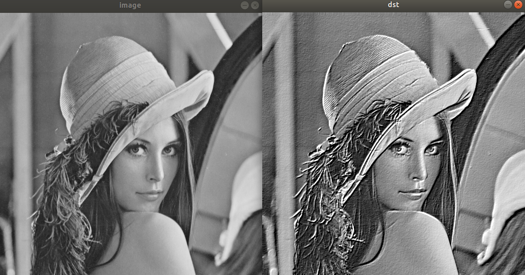
// 예제 코드: 엠보싱.
#include <iostream>
#include "opencv2/opencv.hpp"

int main()
{
    cv::Mat src = cv::imread("./resources/lenna.bmp",cv::IMREAD_GRAYSCALE);
    float data[] = {-1,-1,0,-1,0,1,1,1,1};
    cv::Mat kernel(3,3,CV_32FC1,data);
    cv::Mat dst;
    if (src.empty()){
        std::cerr << "Image load failed!" << std::endl;
        return -1;
    }
    cv::filter2D(src,dst,-1,kernel);

    cv::imshow("image",src);
    cv::imshow("dst",dst);
    cv::waitKey();
    cv::destroyAllWindows();
    return 0;
}

예제 코드는 엠보싱을 구현하기 위한 필터 마스크를 생성한 것이며 엠보싱에 대한 정보는 아래 링크에서 확인 가능하다.
https://en.wikipedia.org/wiki/Image_embossing

코드 실행 결과는 아래와 같다.