[부스트캠프 AI Tech 5기] Pre-Course : (6) numpy part II

📖 reshape

• Array의 shape 크기를 변경함, element의 갯수는 동일

test_matrix = [[1,2,3,4],[1,2,5,8]]
np.array(test_matrix).shape

(2, 4)

np.array(test_matrix).reshape(8,)

array([1, 2, 3, 4, 1, 2, 5, 8])

np.array(test_matrix).reshape(8,).shape

(8,)

np.array(test_matrix).reshape(2,4).shape

(2, 4)

np.array(test_matrix).reshape(-1,2).shape

(4, 2)

np.array(test_matrix).reshape(2,2,2)

array([[[1, 2],
        [3, 4],
       [[1, 2],
        [5, 8]]])

np.array(test_matrix).reshape(2,2,2).shape

(2, 2, 2)

📖 flatten

• 다차원 array를 1차원 array로 변환

test_matrix = [[[1,2,3,4], [1,2,5,8]], [[1,2,3,4], [1,2,5,8]]]
np.array(test_matrix).flatten()

array([1, 2, 3, 4, 1, 2, 5, 8, 1, 2, 3, 4, 1, 2, 5, 8])

📖 indexing for numpy array

• list와 달리 이차원 배열에서 [0,0] 표기법을 제공함
• matrix일 경우 앞은 row 뒤는 column을 의미함

a = np.array([[1, 2, 3], [4.5, 5, 6]], int)
test_example

array([1, 2, 3],
	  [4, 5, 6])

test_example[0][0]

1

test_example[0,0]

1

test_example[0,0] = 12 # Matrix 0,0 에 12 할당 
test_example

array([12, 2, 3],
	  [ 4, 5, 6])

test_example[0][0] = 5 # Matrix 0,0 에 5 할당 
test_example[0,0]

5

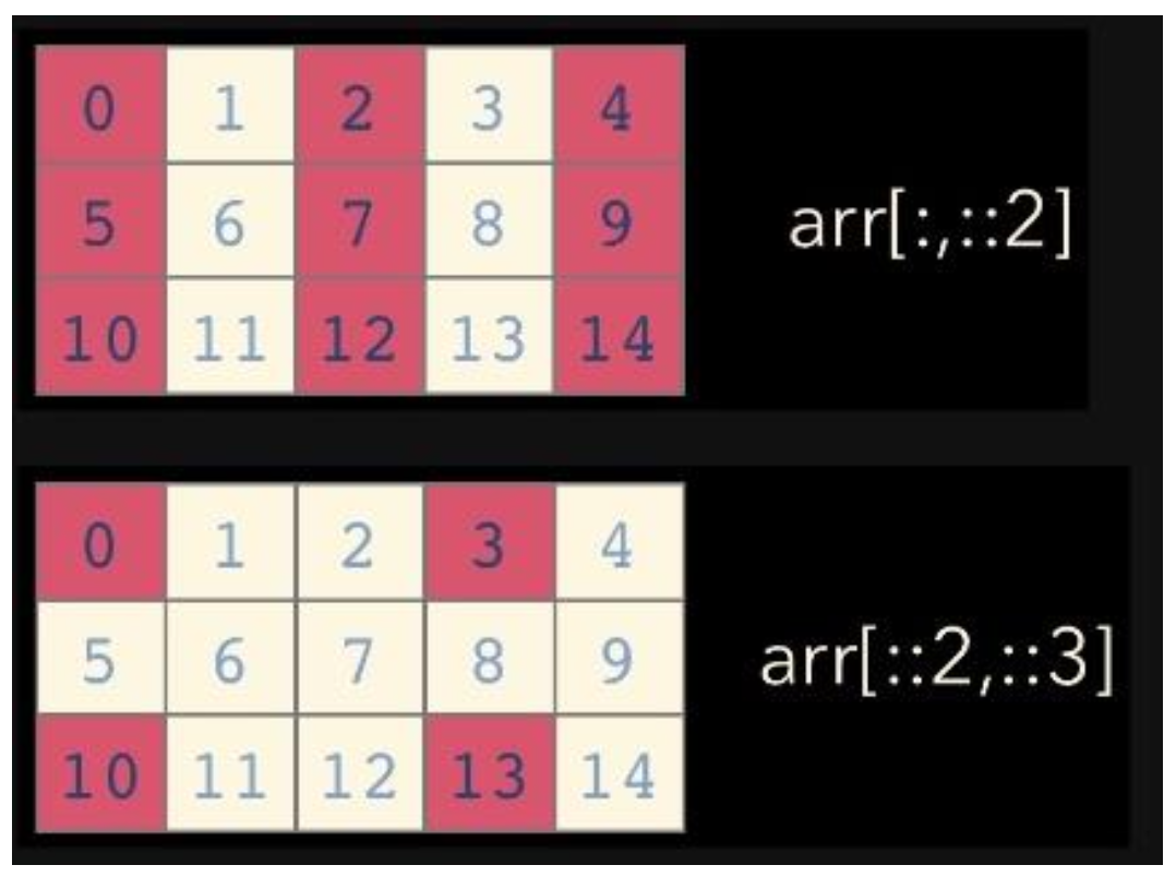
📖 slicing for numpy array

• list와 달리 행과 열 부분을 나눠서 slicing이 가능함
• matrix의 부분 집합을 추출할 때 유용함

# example 1.
a = np.array([[1, 2, 3, 4, 5], [6, 7, 8, 9, 10]], int) 
a[:,2:] # 전체 Row의 2열 이상
a[1,1:3] # 1 Row의 1열 ~ 2열
a[1:3] # 1 Row ~ 2Row의 전체

# example 2.
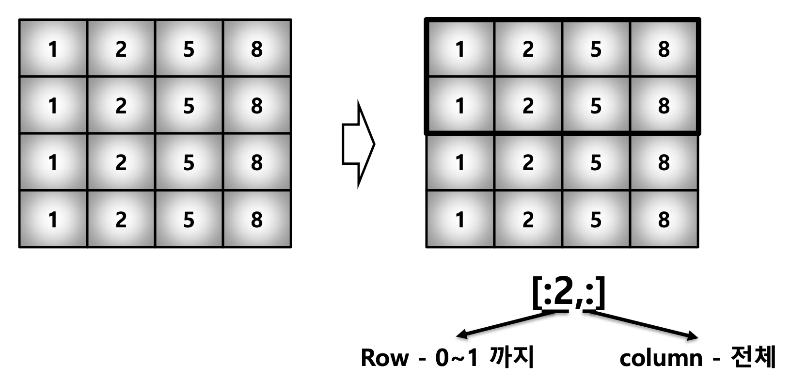
test_example = np.array([[1,2,5,8], [1,2,5,8], [1,2,5,8], [1,2,5,8]], int)
test_example[:2,:]

array([[1,2,5,8],
       [1,2,5,8]])

test_example = np.array([[1,2,3,4,5],[6,7,8,9,10]],int)
test_example[:,2:] # 전체 Row의 2열 이상

array([[3, 4, 5],
       [8, 9, 10]])

test_example[1,1:3] # 1 Row의 1열 ~ 2열

array([7, 8])

test_example[1:3] # 1 Row ~ 2 Row의 전체

array([[ 6, 7, 8, 9, 10]])

(출처 : https://www.slideshare.net/PyData/introduction-to-numpy)

📖 arange

• array의 범위를 지정하여, 값의 list를 생성하는 명령어

# arange : List range와 같은 효과, integer로 0부터 29까지 배열 추출
np.arange(30)

array([ 0, 1, 2, 3, 4, 5, 6, 7, 8, 9, 10, 11, 12, 13, 14, 15, 16,
		17, 18, 19, 20, 21, 22, 23, 24, 25, 26, 27, 28, 29])

# floating point도 표시 가능함
np.arange(0, 5, 0.5)

arary([ 0. , 0.5, 1. , 1.5, 2. , 2.5, 3. , 3.5, 4. , 4.5])

np.arange(30).reshape(5,6)

array([[ 0,  1,  2,  3,  4,  5],
	   [ 6,  7,  8,  9, 10, 11],
       [12, 13, 14, 15, 16, 17],
       [18, 19, 20, 21, 22, 23],
       [24, 25, 26, 27, 28, 29]])

📖 ones, zeros and empty

• zeros : 0으로 가득찬 ndarray 생성

np.zeros(shape, dtype, order)

• ones : 1로 가득찬 ndarray 생성

np.ones(shape, dtype, order)

• empty : shape만 주어지고 비어있는 ndarray 생성
  (memory initialization이 되지 않음)

np.empty(shape, dtype, order)

📖 something_like

• 기존 ndarray의 shape 크기 만큼, 1, 0 또는 empty array를 반환

test_matrix = np.arange(30).reshape(5,6)
np.ones_like(test_matrix)

array([[1, 1, 1, 1, 1, 1],
       [1, 1, 1, 1, 1, 1],
       [1, 1, 1, 1, 1, 1],
       [1, 1, 1, 1, 1, 1],
       [1, 1, 1, 1, 1, 1]])

📖 identity

• 단위 행렬(i 행렬)을 생성함

np.identity(3, dtype=np.int8)

array([[1.,  0.,  0.],
       [0.,  1.,  0.],
       [0.,  0.,  1.]], dtype=np.int8)

np.identity(5)

array([[1., 0., 0., 0., 0.],
       [0., 1., 0., 0., 0.],
       [0., 0., 1., 0., 0.],
       [0., 0., 0., 1., 0.],
       [0., 0., 0., 0., 1.]])

📖 eye

• 대각선이 1인 행렬, k값의 시작 index의 변경이 가능

np.eye(3)

array([[1., 0., 0.],
       [0., 1., 0.],
       [0., 0., 1.]])

np.eye(3,5,k=2)

array([[0., 0., 1., 0., 0.],
       [0., 0., 0., 1., 0.],
       [0., 0., 0., 0., 1.]])

np.eye(N=3, M=5, dtype=np.int8)

array([[1, 0, 0, 0, 0],
       [0, 1, 0, 0, 0],
       [0, 0, 1, 0, 0]], dtype=int8)

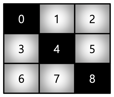
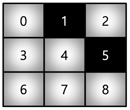
📖 diag

• 대각 행렬의 값을 추출함

matrix = np.arange(9).reshape(3,3)
np.diag(matrix)

array([0, 4, 8])

np.diag(matrix, k=1)

array([1, 5])

📖 random sampling

• 데이터 분포에 따른 sampling으로 array를 생성

# 균등 분포
np.random.uniform(0,1,10).reshape(2,5)

array([[0.09264564, 0.53338537, 0.38126359, 0.8284562 , 0.35628035],
       [0.89126266, 0.62572127, 0.94019628, 0.43529235, 0.47640554]])

# 정규 분포
np.random.normal(0,1,10).reshape(2,5)

array([[ 0.28386836, -0.00801268,  1.55591156, -0.22063183,  0.37625121],
       [ 0.50501499,  0.11751482, -1.28867115,  0.02533356, -0.70049923]])

📖 sum

• ndarray의 element들 간의 합을 구함, list의 sum과 기능 동일

test_array = np.arange(1,11)
test_array

array([ 1,  2,  3,  4,  5,  6,  7,  8,  9, 10])

test_array.sum(dtype=np.float)

55.0

📖 axis

• 모든 operation function을 실행할 때 기준이 되는 dimension 축

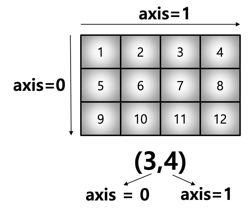
test_array = np.arange(1,13).reshape(3,4)
test_array

array([[ 1,  2,  3,  4],
       [ 5,  6,  7,  8],
       [ 9, 10, 11, 12]])

(test_array.sum(axis=1),test_array.sum(axis=0))

(array([10, 26, 42]), array([15, 18, 21, 24]))

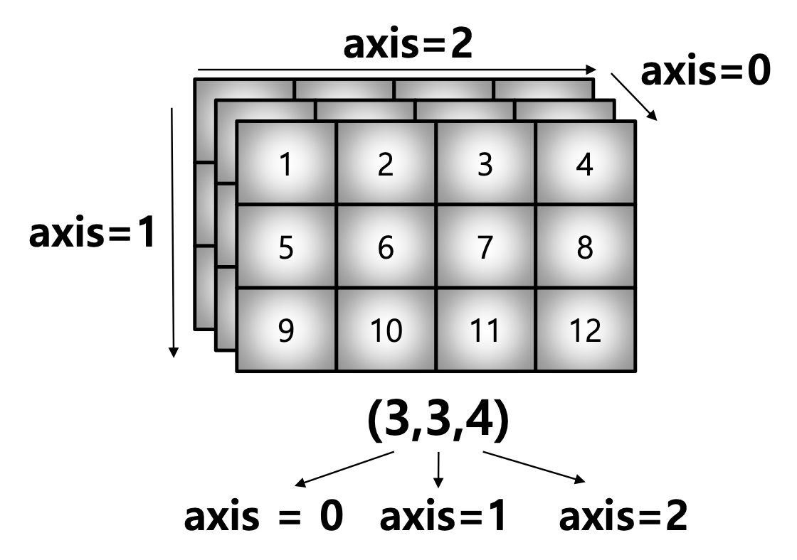
third_order_tensor.sum(axis=2)

array([[10, 26, 42],
       [10, 26, 42],
       [10, 26, 42]])

third_order_tensor.sum(axis=1)

array([[15, 18, 21, 24],
       [15, 18, 21, 24],
       [15, 18, 21, 24]])

third_order_tensor.sum(axis=0)

array([[ 3,  6,  9, 12],
	   [15, 18, 21, 24],
       [27, 30, 33, 36]])

📖 mean & std

• ndarray의 element들 간의 평균 또는 표준 편차를 반환

test_array = np.arange(1,13).reshape(3,4)
test_array

array([[ 1,  2,  3,  4],
       [ 5,  6,  7,  8],
       [ 9, 10, 11, 12]])

test_array.mean(), test_array.mean(axis=0)

(6.5, array([5., 6., 7., 8.]))

test_array.std(), test_array.std(axis=0)

(3.452052529534663, array([3.26598632, 3.26598632, 3.26598632, 3.26598632]))

📖 mathematical functions

• 그 외에도 다양한 수학 연산자를 제공함 (np.something 호출)

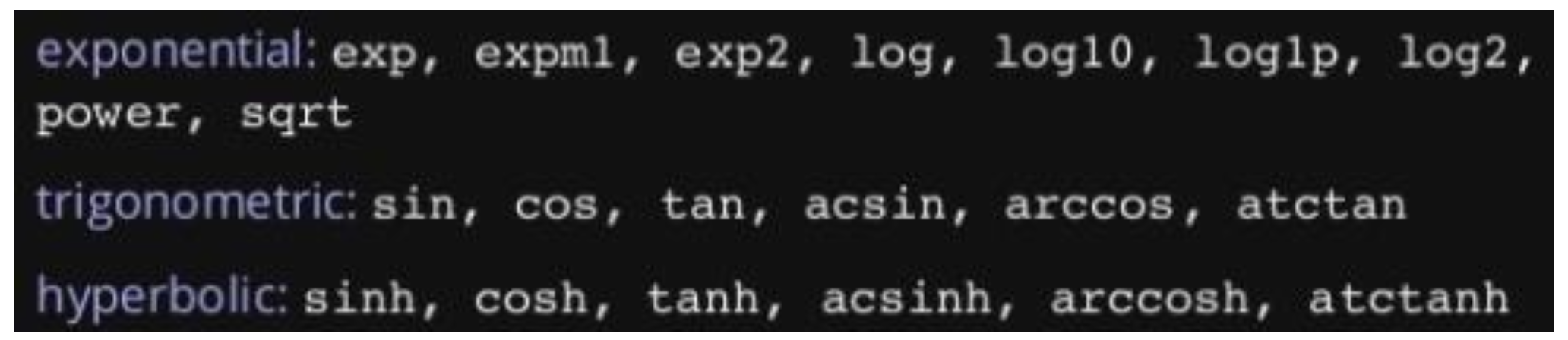
np.exp(test_array), np.sqrt(test_array)

(array([[2.71828183e+00, 7.38905610e+00, 2.00855369e+01, 5.45981500e+01],
        [1.48413159e+02, 4.03428793e+02, 1.09663316e+03, 2.98095799e+03],
        [8.10308393e+03, 2.20264658e+04, 5.98741417e+04, 1.62754791e+05]]),
 array([[1.        , 1.41421356, 1.73205081, 2.        ],
        [2.23606798, 2.44948974, 2.64575131, 2.82842712],
        [3.        , 3.16227766, 3.31662479, 3.46410162]]))

📖 concatnate

• numpy array를 합치는(붙이는) 함수

a = np.array([1, 2, 3])
b = np.array([2, 3, 4])
np.vstack((a,b))

array([[1, 2, 3],
       [2, 3, 4]])

a = np.array([[1], [2], [3]])
b = np.array([[2], [3], [4]])
np.hstack((a,b))

array([[1, 2],
       [2, 3],
       [3, 4]])

a = np.array([[1, 2, 3]])
b = np.array([[2, 3, 4]])
np.concatenate((a,b), axis=0)

array([[1, 2, 3],
       [2, 3, 4]])

a = np.array([[1, 2],[3, 4]])
b = np.array([[5, 6]])
np.concatenate((a,b.T), axis=1)

array([[1, 2, 5],
       [3, 4, 6]])

📖 Operations b/t arrays

• numpy는 array간의 기본적인 사칙 연산을 지원함

test_a = np.array([[1,2,3],[4,5,6]], float)
test_a + test_a

array([[ 2.,  4.,  6.],
       [ 8., 10., 12.]])

test_a - test_a

array([[0., 0., 0.],
       [0., 0., 0.]])

test_a * test_a

array([[ 1.,  4.,  9.],
       [16., 25., 36.]])

📖 Element-wise operations

• Array간 shape이 같을 때 일어나는 연산

matrix_a = np.arange(1,13).reshape(3,4)
matrix_a * matrix_a

array([[  1,   4,   9,  16],
       [ 25,  36,  49,  64],
       [ 81, 100, 121, 144]])

📖 Dot product

• Matrix의 기본 연산, dot 함수 사용

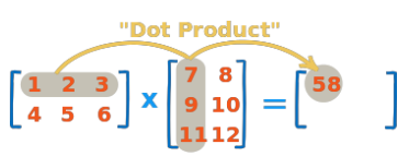
test_a = np.arange(1,7).reshape(2,3)
test_b = np.arange(7,13).reshape(3,2)
test_a.dot(test_b)

array([[ 58,  64],
       [139, 154]])

📖 transpose

• transpose 또는 T attribute 사용

test_a.transpose()

array([[1, 4],
       [2, 5],
       [3, 6]])

test_a.T

array([[1, 4],
       [2, 5],
       [3, 6]])

test_a.T.dot(test_a)

array([[17, 22, 27],
       [22, 29, 36],
       [27, 36, 45]])

📖 broadcasting

• Shape이 다른 배열 간 연산을 지원하는 기능

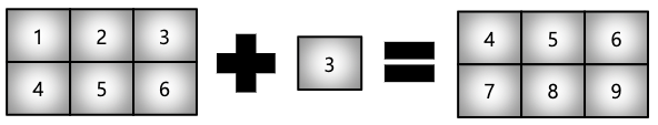
test_matrix = np.array([[1,2,3],[4,5,6]], float)
scalar = 3
# Matrix - Scalar 덧셈
test_matrix + scalar

array([[4., 5., 6.],
       [7., 8., 9.]])

# Matrix - Scalar 뺄셈
test_matrix - scalar

array([[-2., -1.,  0.],
       [ 1.,  2.,  3.]])

# Matrix - Scalar 곱셈
test_matrix * 5

array([[ 5., 10., 15.],
       [20., 25., 30.]])

# Matrix - Scalar 나눗셈
test_matrix / 5

array([[0.2, 0.4, 0.6],
       [0.8, 1. , 1.2]])

# Matrix - Scalar 몫
test_matrix // 0.2

array([[ 4.,  9., 14.],
       [19., 24., 29.]])

# Matrix - Scalar 제곱
test_matrix ** 2

array([[ 1.,  4.,  9.],
       [16., 25., 36.]])

• Scalar - vector 외에도 vector - matrix 간의 연산도 지원

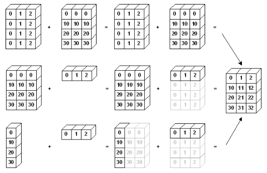
test_matrix = np.arange(1,13).reshape(4,3)
test_vector = np.arange(10,40,10)
test_matrix + test_vector

array([[11, 22, 33],
       [14, 25, 36],
       [17, 28, 39],
       [20, 31, 42]])

📖 numpy performance #1

• timeit : jupyter 환경에서 코드의 퍼포먼스를 체크하는 함수

def sclar_vector_product(scalar, vector):
	result = []
	for value in vector:
    	result.append(scalar * value)
	return result

iternation_max = 100000000

vector = list(range(iternation_max))
scalar = 2

%timeit sclar_vector_product(scalar, vector) # for loop을 이용한 성능
%timeit [scalar * value for value in range(iternation_max)] # list comprehension을 이용한 성능
%timeit np.arange(iternation_max) * scalar # numpy를 이용한 성능

📖 numpy performance #2

• 일반적으로 속도는 아래 순
  for loop < list comprehension < numpy
• 100,000,000번의 loop이 돌 때, 약 4배 이상의 성능 차이를 보임
• Numpy는 C로 구현되어 있어, 성능을 확보하는 대신 파이썬의 가장 큰 특징인 dynamic typing을 포기함
• 대용량 계산에서는 가장 흔히 사용됨
• Concatenate처럼 계산이 아닌, 할당에서는 연산 속도의 이점이 없음

<이 게시물은 최성철 교수님의 numpy 강의 자료를 참고하여 작성되었습니다.>

본 포스트의 학습 내용은 [부스트캠프 AI Tech 5기] Pre-Course 강의 내용을 바탕으로 작성되었습니다.
부스트캠프 AI Tech 5기 Pre-Course는 일정 기간 동안에만 운영되는 강의이며,
AI 관련 강의를 학습하고자 하시는 분들은 부스트코스 AI 강좌에서 기간 제한 없이 학습하실 수 있습니다.
(https://www.boostcourse.org/)