ch4.7 LightGBM
LightGBM은 XGBoost와 함께 부스팅 계열 알고리즘에서 가장 많이 사용된다. XGBoost는 GBM 보다는 빠르지만 여전히 학습 시간이 오래 걸린다는 단점이 있다. LightGBM은 이러한 학습 시간을 개선한 알고리즘이라 할 수 있겠다. (메모리 사용량도 적음!)
-
장점
- 더 빠른 학습과 예측 수행 시간
- 메모리 사용량이 적음
- XGBoost와 예측 성능에서 큰 차이가 없음
- 카테고리형 피처의 자동 변환과 최적 분할
(원-핫 인코딩을 사용하지 않아도 피처를 최적으로 분할함)
-
단점
- 적은 데이터셋에 대해서는 과적합 우려가 있음 (기준 - 공식 문서에 의하면 약 1 만건 이하의 데이터셋)
일반적인 GBM 계열의 트리 분할 방법은 트리의 깊이를 효과적으로 줄이기 위해 '균형 트리 분할 방식'을 사용한다. (오버피팅에 더 강한 구조이기 때문) 이러한 방식은 균형을 맞추기 위한 시간이 필요하다는 상대적인 단점이 존재한다.
LightGBM은 '균형 트리 분할 방식' (Level Wise) 이 아닌 '리프 중심 트리 분할 방식' (Leaf Wise) 을 사용한다. 최대 손실 값을 가지는 리프 노드를 지속적으로 분할하면서 트리의 깊이가 깊어지고 비대칭적인 규칙 트리가 생성되는 것이 특징이다.
결국 학습을 반복할수록 균형 트리 분할 방식보다 예측 오류 손실을 최소화할 수 있다는 것이 해당 알고리즘의 사상이라 할 수 있겠다.
ch4.7 사이킷런 래퍼 LightGBM 하이퍼 파라미터
-
n_estimators
- 반복을 수행하려는 트리의 개수
- 기본값은 100
-
learning_rate
- 기본값은 0.1
-
max_depth
- Depth wise 방식이 아닌 Leaf Wise 방식이므로 깊이가 상대적으로 더 깊다는 점을 참고
- 0보다 작은 값을 지정하면 깊이에 제한이 없음
- 기본값은 -1
-
min_child_samples
- 결정트리의 min_samples_leaf와 같은 파라미터
- 기본값은 20
-
num_leaves
- 하나의 트리가 가질 수 있는 최대 리프 개수
- 기본값은 31
-
위에서 언급한 파라미터 외에도 reg_lambda, reg_alpha, feature_fraction 등 다양한 하이퍼 파라미터가 존재함
ch4.7 LightGBM 과적합 감소 방법
LightGBM 모델 복잡도를 제어하는 주요 파라미터는 아래와 같다. 세 파라미터 모두 값이 커질수록 정확도가 올라갈 수 있지만 모델 복잡도가 커져 과적합 영향도 또한 커진다.
- num_leaves
- min_child_samples
- max_depth
ch4.7 LightGBM 실습
- 데이터 로드 (위스콘신 유방암 예측)
from lightgbm import LGBMClassifier

import pandas as pd
import numpy as np
from sklearn.datasets import load_breast_cancer
from sklearn.model_selection import train_test_split
dataset = load_breast_cancer()
dataset## dataframe 생성
cancer_df = pd.DataFrame(data=dataset.data, columns=dataset.feature_names)## dataframe에 레이블 열 추가
cancer_df['target'] = dataset.target- 모델 로드
## dataframe에서 feature과 label 구분
X_features = cancer_df.iloc[:, :-1]
y_label = cancer_df.iloc[:, -1]

## data split => train / test
X_train, X_test, y_train, y_test = train_test_split(X_features, y_label, test_size=0.2, random_state=156)

## data split => train => train / val
X_tr, X_val, y_tr, y_val = train_test_split(X_train, y_train, test_size=0.1, random_state=156)
## lgbm model
lgbm_wrapper = LGBMClassifier(n_estimators=400, learning_rate=0.05) ## 400번 epochs, lr = 0.05 지정## learly stopping
evals = [(X_tr, y_tr), (X_val, y_val)]- 모델 학습
## model_training => early stopping으로 인해 조기 중단됨
lgbm_wrapper.fit(X_tr, y_tr,
                 early_stopping_rounds=50,
                 eval_metric="logloss",
                 eval_set=evals,
                 verbose=True
)- 모델 평가
preds = lgbm_wrapper.predict(X_test)
pred_proba = lgbm_wrapper.predict_proba(X_test)
pred_proba = pred_proba[:, 1]## 모델 성능 평가 함수 선언
from sklearn.metrics import accuracy_score, confusion_matrix, precision_score, recall_score, f1_score, roc_auc_score
def get_clf_eval(y_test, pred=None, pred_proba=None):
confusion = confusion_matrix(y_test, pred)
accuracy = accuracy_score(y_test, pred)
precision = precision_score(y_test, pred)
recall = recall_score(y_test, pred)
f1 = f1_score(y_test, pred)
roc_auc = roc_auc_score(y_test, pred_proba)
print('오차 행렬')
print(confusion)
print('정확도: {0:.4f}, 정밀도: {1:.4f}, 재현율: {2:.4f}, F1: {3:.4f}, AUC: {4:.4f}'.format(accuracy, precision, recall, f1, roc_auc))get_clf_eval(y_test, preds, pred_proba)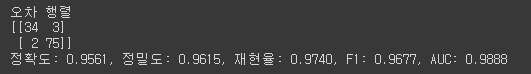
- 피처 중요도 확인
import matplotlib.pyplot as plt
import seaborn as sns
%matplotlib inline

ftr_importances_values = lgbm_wrapper.feature_importances_ ## feature_importances_
ftr_importances = pd.Series(ftr_importances_values, index=X_train.columns)
ftr_top20 = ftr_importances.sort_values(ascending=False)[:20]

plt.figure(figsize=(8, 6))
plt.title('Feature importances Top 20')
sns.barplot(x=ftr_top20, y=ftr_top20.index)
plt.show()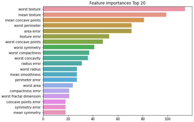

행복한 소히의 이것저것