[논문 정리] TabNet: Attentive Interpretable Tabular Learning

shyoon·2023년 7월 30일

논문정리

목록 보기

1/11

1. Introduction

해당 논문이 발췌될 때의 양상은, 딥러닝 기반 모델들이 이미지, 텍스트, 오디오 등의 데이터 타입들 에서는 뛰어난 성공을 보여주고 있었다. 하지만, Tabular data(정형 데이터)에서는 tree 기반의 다양한 앙상블 모델들이 여전히 우세한 면을 보이고 있었다. 이에는 아래와 같은 대표적인 세 가지 이유가 있다.

트리 기반 모델들이 초평면(hyperplane) 경계의 manifolds에서 효율적인데, Tabular data 가 보통 이러한 특성을 갖기 때문

트리 기반 앙상블 모델들이 높은 해석력과 사후 분석 method들을 가지기 때문

트리 기반 모델들의 학습 속도가 빠르고, 이전에 제안된 DNN 모델들이 tabular dataset에 잘 적합되지 않았기 때문

이에 저자들은 딥러닝 모델을 Tabular dataset에 적용해야할 필요성을 주장하였다.

정형 데이터와 다른 타입의 데이터들(이미지)을 함께 encoding 하는 것이 가능하다.

Feature Engineering의 필요성을 완화해 준다.

Streaming data로 부터의 학습이 가능하다.

딥러닝의 end-to-end 모델은 다양한 applicaiton scenarios(data-efficient domain adaptation, generative modeling, semi-supervised learning)을 가능케 해준다.

이어서 위와 같은 장점들을 활용하기 위해 저자들이 새로 제안한 canonical DNN 구조의 contributions는 다음과 같다.

TabNet은 어떠한 전처리 과정 없이 raw tabular data를 input하여 gradient descent-based optimization을 이용하여 end-to-end learning을 할 수 있게 함.

TabNet은 sequential attention을 이용하여 각 의사결정 단계에서 어느 feature가 중요하게 작용하였는 지 알 수 있게 하여 해석력을 높인다. 이러한 feature selection은 개별 instance별로 따로따로 시행한다.

이러한 점은 기존의 분류, 회귀 모델보다 못하지 않은 성능을 보이고, 각 feature의 중요성과 그것이 어떻게 결합되었는지를 보여주는 local 해석력과, 각 feature가 trained model에 얼마나 기여했는지를 정량화 해주는 global 해석력을 부여한다.

정형 데이터에서는 처음으로 unsupervised pre-training을 이용해 마스킹 된 feature를 예측하는 데 상당한 성능 향상을 보였다.

Feature Selection

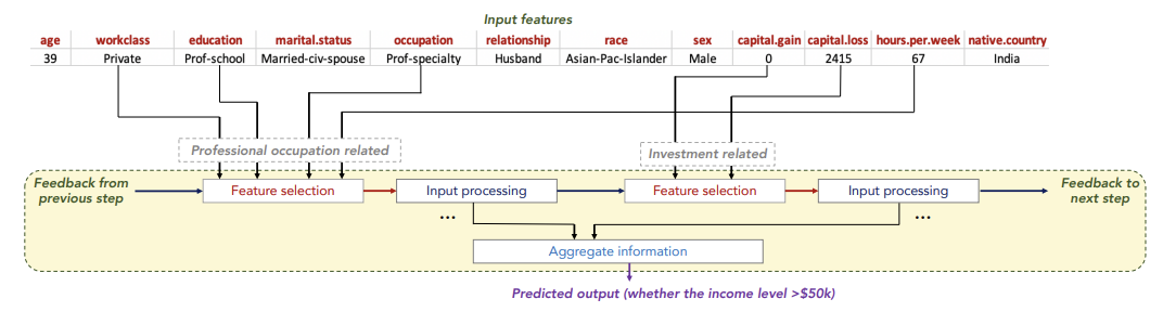
TabNet에서는 sparse feature selection을 제안하여 sequential하게 feature selection을 진행. 각 step 별로 중요한 feature를 파악 가능하여 instance-wise 한 feature selection이 가능하고, 이는 local interpretability를 부여한다. 그리고 당연히 전체 데이터에 대한 feature 중요도를 파악하여 global interpretability도 확보할 수 있다.

위 그림은 어느 사람의 소득을 예측하는 과정인데, 첫 step에서는 직업과 관련한 feature 위주로 학습하고, 다음 step에서는 소득과 관련한 feature 위주로 학습하는 것을 확인할 수 있다.

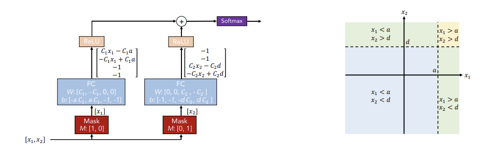
Integration of DNNs into DTs
좌측 그림은 conventional DNN blocks 이다. 좌측 mask block을 보면 첫 번째 계수만 1이어서 첫 번째 변수들에 대해서만 학습하고, 우측 mask block에서는 두번째 변수들에 대해서만 학습한다. 그 결과 선택된 변수들로 결정 경계를 만들어가고, 이를 통해 딥러닝 모델이 트리 모델처럼 학습이 가능하다.

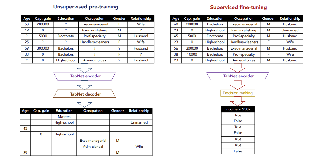
Self-supervised learning
TabNet에서는 Self-supervised learning을 위해 무작위로 masking 된 값들을 예측하는 비지도학습을 수행. 이를 위해 encoder에 decoder가 추가 되는 autoencoder 구조를 지니고, 실제 데이터 셋에 결측값이 있었다면, 위 방법을 통해 값들을 채워준다. 이렇게 완성된 데이터셋으로 supervised fine-tuning을 진행하여 성능을 향상시킨다.

3. Structure

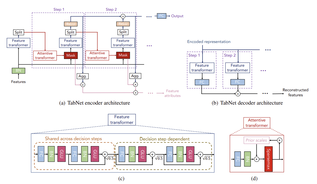
전체적인 TabNet의 구조

⇨ 간략하게 말하자면, Feature Transformer에서는 feature processing 과정이, Attentive Transformer에서는 feature selection 과정이 진행된다고 보면 된다.

Attentive Transformer

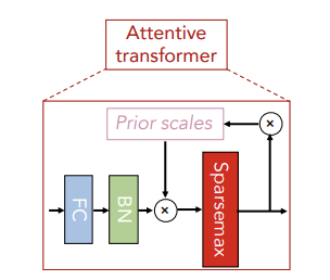
Feature Selection을 수행하는 구조로 학습 가능한 Mask를 출력한다.
이전 step에서 가공되어 input된 $a[i-1]$ 이 FC(Fully Connected) layer, BN(Batch Normalization) layer을 거치며 $h_i(a[i-1])$ 이 되고, $P[i-1]$ 을 곱해준 다음 Sparsemax 적용 해 준다. 이 때, $P[i-1]$ 은 이전 step의 Prior Scales로 이전 decision step에서 선택되었던 feature의 재선택 비율을 조정해준다.

P[i] = \prod_{j=1}^j(\gamma-M[j])

$M[j]$ 는 이전 step에서 생성된 mask고, $\gamma$ 는 조정 가능한 하이퍼 파라미터로 1 이상인 수이다. 이 때 $\gamma$ 값을 1로 설정하면 이전 단계에서 중요했던 컬럼의 마스크 값은 1이었기에 빼주면 0이 되고 이를 다음 step의 $h_i(a[i-1])$ 에 곱해주게 되므로, 이전에 선택되었던 변수는 다시 선택되지 않을 확률이 높아진다.

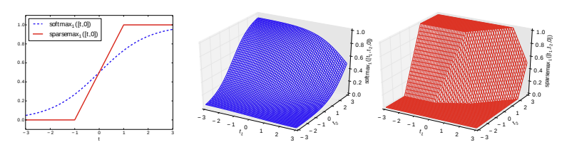
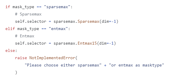
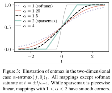
※ Sparsemax

softmax보다 sparsity를 고려한 활성화 함수로 softmax처럼 0과 1 사이의 값으로 반환되지만 더 극적이다. 선택된 feature 가중치는 softmax보다 훨씬 1에 가까운 값들로, 선택되지 않은 feature 가중치는 0에 훨씬 가까운 값들로 반환된다.

제공된 TabNet 깃허브 코드를 살펴보면 Entmax를 쓰는 경우도 확인할 수 있는데, $\alpha$ 값을 조정 가능하여 1이면 softmax, 2면 sparsemax와 같아 $\alpha$ 값이 클수록 가파라 진다고 보면 될 것 같다.

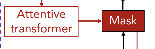
이렇게 Attentive Transformer의 결과로 출력된 마스크를 이전 step의 feature에 곱해줌으로써 soft feature selection이 진행되고, 이는 다시 다음 단계의 Feature Transformer의 input이 된다.

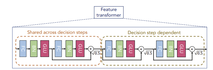
Feature Transformer

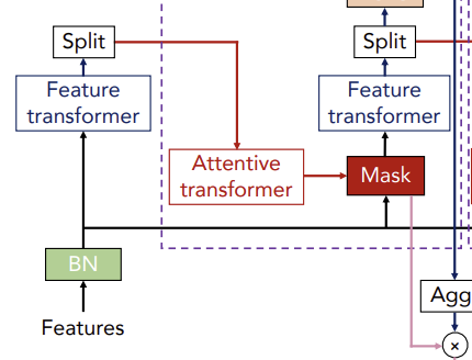
Feature processing을 수행하는 구조로 마스킹 과정을 거친 masked feature들을 embedding 해 준다.

첫 step의 input은 Batch Normalization을 거친 feature이고, 그 이후 step의 input은 masking 과정을 거친 feature들이다.

Feature Transformer는 두 종류의 블럭으로 구성되는데, 좌측의 Shared across decision steps와 우측의 Decision step dependent이다. 좌측은 전체 decision step에서 파라미터를 공유하고, 우측은 해당 step에서의 파라미터만 이용한다.

각 block은 공통적으로 Fully Connected Layer - Batch Normalization - Gated Linear Unit 연결 구조를 지닌다. 이 때 input features를 제외한 BN은 Ghost Batch Normalization을 진행하여 학습 속도를 향상시켰고, 블럭마다 $\sqrt{0.5}$ 곱해주어 분산을 작게 해준다. 그 결과 D차원으로 임베딩 된 features( $f$ )를 출력한다.

Split & ReLU

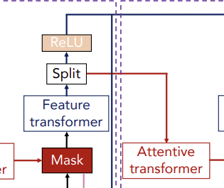
이렇게 결과로 나온 $f$ 를 $d[i]$ , $a[i]$ 로 Split 하여 $d[i]$ 에는 ReLU를 적용하는데 그 결과는 step[ $i$ ] 에서의 feature importance를 의미한다. $a[i]$ 는 다음 step을 위한 input이 된다. 최종적으로 ReLu를 적용한 $d[i]$ 들을 합해주어 최종적인 feature attributes를 생성한다.

Decoder

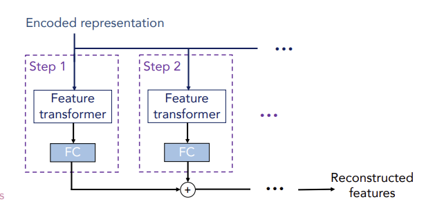
Self-Supervised Learning을 위해 필요한 구조로 Encoder의 각 step마다 feature transformer의 output인 $d[i]$ 를 input으로 받아서 Feature Transformer, FC layer를 거쳐서 모든 step의 결과를 최종적으로 합한 features를 출력한다. 이러한 encoder-decoder 구조를 통해 Unsupervised pre-training과정을 진행하고, 그 결과를 가지고 Supervised fine-tuning을 진행하여 성능을 향상시켰다.

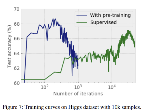
위와 같이 pre-training을 진행하지 않은 경우보다 훨씬 빠르게 수렴하는 결과를 보인다.

4. Interpretability

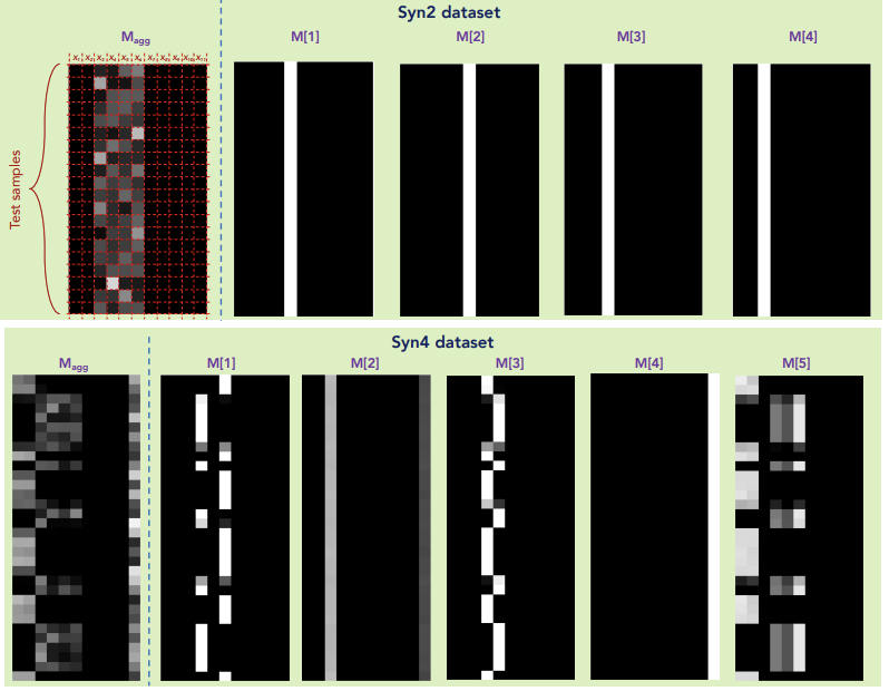
위의 Syn2 데이터 셋은 샘플(행) 별로 중요 feature의 차이가 없는 데이터 셋이고, Syn4 데이터 셋은 샘플 별로 중요 feature가 다른 데이터 셋이다. Syn4 결과에서는 행 마다 흰 부분인 열(중요한 feature)이 다른 것을 확인할 수 있다. 따라서 각 step 별로 중요 feature들을 확인할 수 있고, 이를 aggregate하여 전체적인 feature 중요도 또한 확인할 수 있다.

5. Experiment

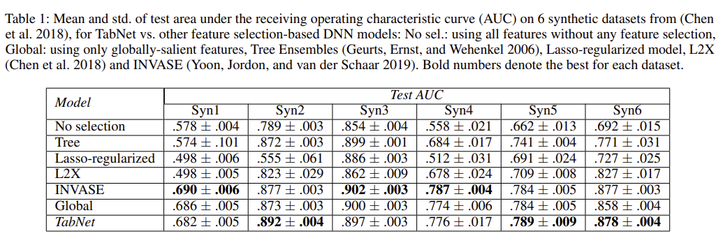
(Syn 1~6 은 저자들이 임의로 생성한 데이터 셋이다.)
위 테이블에서 Syn 1~3은 샘플 별로 중요 feature 차이가 없는 데이터 셋이고, Syn 4~6은 샘플 별로 중요 feature 차이가 있는 데이터 셋이다. 위의 정확도 결과는 중요 feature 차이 없는 데이터 셋에서는 다른 모델들과 비교했을 때 큰 성능 차이가 없지만, 그렇지 않은 데이터 셋에서 좋은 성능을 띠는 것을 보여주고 있다.

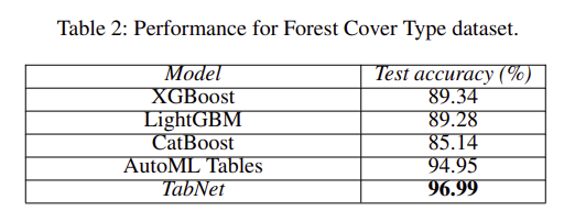
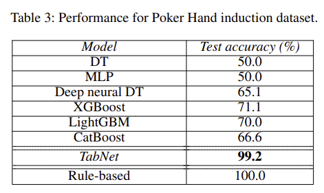
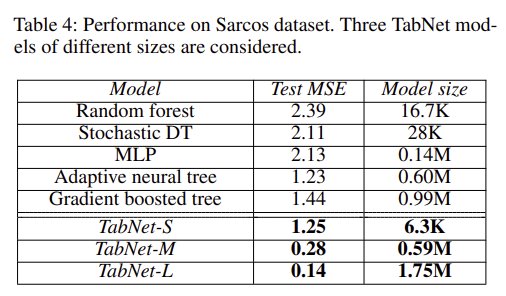
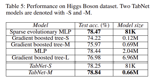
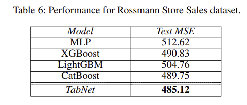
그 외에도 위 처럼 다양한 real-world 데이터 셋들에 적용했을 때 모델이 비교적 가벼움에도 불구하고 무거운 모델들보다 좋은 성능을 보이는 실험 결과들을 보여주고 있다.

6. 코드 실습 및 리뷰

저자의 깃허브에 올라와 있는 TabNet 실습 sample code를 그대로 진행 해보았다.

from pytorch_tabnet.tab_model import TabNetClassifier

import torch
from sklearn.preprocessing import LabelEncoder
from sklearn.metrics import roc_auc_score

import pandas as pd
import numpy as np
np.random.seed(0)

import scipy

from fastai.imports import *
import os
import wget
from matplotlib import pyplot as plt
%matplotlib inline

필요한 패키지 및 라이브러리 import

url = "https://archive.ics.uci.edu/ml/machine-learning-databases/adult/adult.data"
dataset_name = 'census-income'
out = Path(os.getcwd()+'/data/'+dataset_name+'.csv')

out.parent.mkdir(parents=True, exist_ok=True)
if out.exists():
    print("File already exists.")
else:
    print("Downloading file...")
    wget.download(url, out.as_posix())

census-income 데이터 셋 다운로드

train = pd.read_csv(out)
target = ' <=50K'
if "Set" not in train.columns:
    train["Set"] = np.random.choice(["train", "valid", "test"], p =[.8, .1, .1], size=(train.shape[0],))

train_indices = train[train.Set=="train"].index
valid_indices = train[train.Set=="valid"].index
test_indices = train[train.Set=="test"].index

데이터를 불러오고 split

from pandas.core.arrays import categorical

nunique = train.nunique()
types = train.dtypes

categorical_columns = []
categorical_dims = {}

for col in train.columns:
  if types[col] == 'object' or nunique[col] < 200:
    print(col, train[col].nunique())
    l_enc = LabelEncoder()
    train[col] = train[col].fillna("VV_likely")
    train[col] = l_enc.fit_transform(train[col].values)
    categorical_columns.append(col)
    categorical_dims[col] = len(l_enc.classes_)
  else:
    train.fillna(train.loc[train_indices, col].mean(), inplace=True)
    
# check that pipeline acceptss trings
train.loc[train[target]==0, target] = 'wealthy'
train.loc[train[target]==1, target] = 'not_wealthy'

unused_feat = ['Set']
features = [col for col in train.columns if col not in unused_feat+[target]]
cat_idxs = [i for i, f in enumerate(features) if f in categorical_columns]
cat_dims = [categorical_dims[f] for i, f in enumerate(features) if f in categorical_columns]

범주형 변수를 encoding 하고 정의 해 주는 과정. 데이터 타입이 'object'가 아니어도 unique 값 수가 200보다 작아도 범주형으로 처리한다. numerical 변수의 결측치는 평균으로 대체

tabnet_params = {"cat_idxs":cat_idxs,
                 "cat_dims":cat_dims,
                 "cat_emb_dim":2,
                 "optimizer_fn":torch.optim.Adam,
                 "optimizer_params":dict(lr=2e-2),
                 "scheduler_params":{"step_size":50, "gamma":0.9},
                 "scheduler_fn":torch.optim.lr_scheduler.StepLR,
                 "mask_type":'entmax',
                 "grouped_features": grouped_features}

clf = TabNetClassifier(**tabnet_params)

X_train = train[features].values[train_indices]
y_train = train[target].values[train_indices]

X_valid = train[features].values[valid_indices]
y_valid = train[target].values[valid_indices]

X_test = train[features].values[test_indices]
y_test = train[target].values[test_indices]

파라미터 설정 및 TabNet Classifier 선언

max_epochs = 30

clf.fit(
    X_train=X_train, y_train=y_train,
    eval_set=[(X_train, y_train), (X_valid, y_valid)],
    eval_name=['train', 'valid'],
    eval_metric=['auc'],
    max_epochs=max_epochs, patience=20,
    batch_size=1024, virtual_batch_size=128,
    num_workers=0,
    weights=1,
    drop_last=False,
)

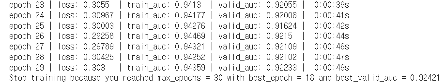
max_epoch을 임의로 30으로 설정하고 모델링 진행 해 보았다.

preds = clf.predict_proba(X_test)
test_auc = roc_auc_score(y_score=preds[:, 1], y_true=y_test)

preds_valid = clf.predict_proba(X_valid)
valid_auc = roc_auc_score(y_score=preds_valid[:, 1], y_true=y_valid)

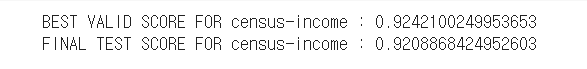
print(f"BEST VALID SCORE FOR {dataset_name} : {clf.best_cost}")
print(f"FINAL TEST SCORE FOR {dataset_name} : {test_auc}")

예측 정확도는 0.921 정도 나온 것을 확인할 수 있다.

위 그림은 1, 2, 3 step mask의 중요 feature들을 시각화 한 것.

XGB와 비교

from xgboost import XGBClassifier

clf_xgb = XGBClassifier(max_depth=8,
                        learning_rate=0.1,
                        n_estimators=1000,
                        verbosity=0,
                        silent=None,
                        objective='binary:logistic',
                        booster='gbtree',
                        n_jobs=-1,
                        nthread=None,
                        gamma=0,
                        min_child_weight=1,
                        max_delta_step=0,
                        subsample=0.7,
                        colsample_bytree=1,
                        colsample_bylevel=1,
                        colsample_bynode=1,
                        reg_alpha=0,
                        reg_lambda=1,
                        scale_pos_weight=1,
                        base_score=0.5,
                        random_state=0,
                        seed=None)

clf_xgb.fit(X_train, y_train,
            eval_set=[(X_valid, y_valid)],
            early_stopping_rounds=40,
            verbose=10)

preds = np.array(clf_xgb.predict_proba(X_valid))
valid_auc = roc_auc_score(y_score=preds[:,1], y_true=y_valid)
print(valid_auc)

preds = np.array(clf_xgb.predict_proba(X_test))
test_auc = roc_auc_score(y_score=preds[:, 1], y_true=y_test)
print(test_auc)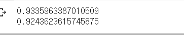

XGB의 예측 정확도는 0.924가 나왔다.

Comment

실습에서는 시간 관계상 TabNet과 XGB의 하이퍼 파라미터 튜닝을 많이 진행 해 보지 못하고 예제 코드 그대로 썼는데 일단 결과적으로 봤을 때 큰 차이는 안나지만 근소하게 XGB의 예측 정확도가 조금 더 높게 나왔다. 시간 될 때 더 자세히 실습 진행 해 보아야 할 것 같다.
최근 캐글이나 데이콘 등에서 Tabular dataset에 좋은 성적을 보이며 다른 트리 기반 앙상블 모델에 비해 장점들을 많이 가지고 있지만 아직 모든 데이터 셋에 대해 이들보다 좋은 성능을 보이는 것은 아니라고 한다. Variant TabNet 기법에 대해서 추가 공부가 필요할 것 같다.