이미지를 분류하는 Classifer를 구현하기 전에 먼저 데이터에 대해 알아보자.
평소에 우리가 이미지, 텍스트, 오디오, 비디오 데이터를 상대할때, 우리는 데이터를 넘파이 배열로 불러오는 standard한 파이썬 패키지들을 사용하면 된다.
➡ 그 다음 이 넘파이 배열을 torch.*Tensor로 변환하면 된다.
데이터별 유용한 파이썬 패키지
- 이미지:
Pillow,OpenCV - 오디오:
scipy,librosa - 텍스트:
raw Python or Cython based loading,NLTK,SpaCy
특히 비전에서는 torchvision 패키지를 생성한다.
torchvision 패키지 안에는 다음이 포함된다.
- data loaders for common datasets(ImageNet, CIFAR10, MNIST, ...)
- data transformers for images, viz.,
torchvision.datasets,torch.utils.data.DataLoader
👍 이 패키지로 인해 엄청난 편리성을 얻을 수 있고, boilerplate code를 쓰지 않아도 된다는 장점이 있다.
이미지 분류 구현하기
CIFAR10 데이터셋을 사용해보자.
-
클래스: ‘airplane’, ‘automobile’, ‘bird’, ‘cat’, ‘deer’, ‘dog’, ‘frog’, ‘horse’, ‘ship’, ‘truck’
-
이미지 크기: 3x32x32 (3-channel color images of 32x32 pixels)
이미지 분류 구현 과정
- Load and normalize the CIFAR10 training and test datasets using torchvision
- Define a Convolutional Neural Network
- Define a loss function
- Train the network on the training data
- Test the network on the test data
1. Load and Normalize CIFAR10
torchvision을 이용하면 CIFAR10 데이터셋을 아주 쉽게 로드할 수 있다.
import torch
import torchvision
import torchvision.transforms as transforms
torchvision 데이터셋의 결과는 [0, 1]의 범위를 가지는 PILImage 이미지이다.
➡ 이 결과를 [-1, 1]의 정규화된 범위를 가지는 tensor로 변환한다.
transform = transforms.Compose(
    [transforms.ToTensor(),
     transforms.Normalize((0.5, 0.5, 0.5), (0.5, 0.5, 0.5))])

batch_size = 4

trainset = torchvision.datasets.CIFAR10(root='./data', train=True,
                                        download=True, transform=transform)
trainloader = torch.utils.data.DataLoader(trainset, batch_size=batch_size,
                                          shuffle=True, num_workers=2)

testset = torchvision.datasets.CIFAR10(root='./data', train=False,
                                       download=True, transform=transform)
testloader = torch.utils.data.DataLoader(testset, batch_size=batch_size,
                                         shuffle=False, num_workers=2)

classes = ('plane', 'car', 'bird', 'cat',
           'deer', 'dog', 'frog', 'horse', 'ship', 'truck')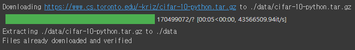
학습 이미지 중 일부를 출력해보자. (재미로..ㅎㅎ)
import matplotlib.pyplot as plt
import numpy as np

# functions to show an image


def imshow(img):
    img = img / 2 + 0.5     # unnormalize
    npimg = img.numpy()
    plt.imshow(np.transpose(npimg, (1, 2, 0)))
    plt.show()


# get some random training images
dataiter = iter(trainloader)
images, labels = dataiter.next()

# show images
imshow(torchvision.utils.make_grid(images))
# print labels
print(' '.join(f'{classes[labels[j]]:5s}' for j in range(batch_size)))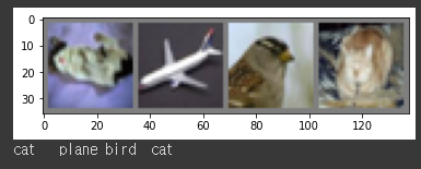
2. Define a Convolutional Neural Network
3-channel 이미지를 take하는 neural network를 만들자!
import torch.nn as nn
import torch.nn.functional as F

class Net(nn.Module):
    def __init__(self):
        super().__init__()
        self.conv1 = nn.Conv2d(3, 6, 5)
        self.pool = nn.MaxPool2d(2, 2)
        self.conv2 = nn.Conv2d(6, 16, 5)
        self.fc1 = nn.Linear(16 * 5 * 5, 120)
        self.fc2 = nn.Linear(120, 84)
        self.fc3 = nn.Linear(84, 10)

    def forward(self, x):
        x = self.pool(F.relu(self.conv1(x)))
        x = self.pool(F.relu(self.conv2(x)))
        x = torch.flatten(x, 1) # flatten all dimensions except batch
        x = F.relu(self.fc1(x))
        x = F.relu(self.fc2(x))
        x = self.fc3(x)
        return x


net = Net()
3. Define a Loss function and optimizer
Classification Cross-Entropy loss & SGD with momentum을 사용해보자!
import torch.optim as optim

criterion = nn.CrossEntropyLoss()
optimizer = optim.SGD(net.parameters(), lr=0.001, momentum=0.9)
4. Train the Network
data iterator를 반복시키고, 네트워크에 input을 넣고 최적화한다.
for epoch in range(2):  # loop over the dataset multiple times

    running_loss = 0.0
    for i, data in enumerate(trainloader, 0):
        # get the inputs; data is a list of [inputs, labels]
        inputs, labels = data

        # zero the parameter gradients
        optimizer.zero_grad()

        # forward + backward + optimize
        outputs = net(inputs)
        loss = criterion(outputs, labels)
        loss.backward()
        optimizer.step()

        # print statistics
        running_loss += loss.item()
        if i % 2000 == 1999:    # print every 2000 mini-batches
            print(f'[{epoch + 1}, {i + 1:5d}] loss: {running_loss / 2000:.3f}')
            running_loss = 0.0

print('Finished Training')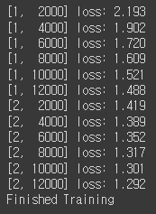
학습한 모델을 저장하자!
PATH = './cifar_net.pth'
torch.save(net.state_dict(), PATH)
5. Test the Network on the Test Data
학습 데이터셋에서 2 passes 동안 네트워크를 학습시켰다. 하지만 네트워크가 학습한 게 있는지 체크해봐야 한다.
➡neural network 결과인 class label을 예측하고, ground-truth와 비교함으로써 체크할 수 있다!
예측이 정확하면 correct prediction 리스트에 해당 샘플을 추가하면 된다!
먼저 테스트 셋을 살펴보자.
dataiter = iter(testloader)
images, labels = dataiter.next()

# print images
imshow(torchvision.utils.make_grid(images))
print('GroundTruth: ', ' '.join(f'{classes[labels[j]]:5s}' for j in range(4)))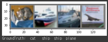
saved model을 다시 로드하자!
(모델 저장과 리로딩이 여기서 중요한 건 아니지만 어떻게 하는지 알기 위해서!)
net = Net()
net.load_state_dict(torch.load(PATH))
neural network가 이 예시들을 어떻게 예측하는지 보자!
outpus는 10개의 클래스에 대한 energy이다.
가장 높은 에너지를 가질수록, 네트워크가 해당 이미지가 특정 클래스에 속한다는 예측이 강해진다.
가장 높은 에너지를 가지는 인덱스를 가져와보자!
outputs = net(images)_, predicted = torch.max(outputs, 1)
print('Predicted: ', ' '.join(f'{classes[predicted[j]]:5s}'
for j in range(4)))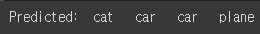
위의 결과창을 보면 결과가 괜찮은 걸 볼 수 있다.
이제 네트워크가 전체 데이터셋에서 어떻게 perform하는지 살펴보자!
correct = 0
total = 0
# since we're not training, we don't need to calculate the gradients for our outputs
with torch.no_grad():
    for data in testloader:
        images, labels = data
        # calculate outputs by running images through the network
        outputs = net(images)
        # the class with the highest energy is what we choose as prediction
        _, predicted = torch.max(outputs.data, 1)
        total += labels.size(0)
        correct += (predicted == labels).sum().item()

print(f'Accuracy of the network on the 10000 test images: {100 * correct // total} %')
10%의 정확도를 가지는 chance(10개의 클래스에서 랜덤으로 한 클래스를 뽑음)보다 더 결과가 좋아보인다.
➡ 네트워크가 무언갈 학습한 것으로 보인다.
어떤 클래스가 성능이 좋고, 어떤 클래스가 성능이 안 좋은지 알아보자!
# prepare to count predictions for each class
correct_pred = {classname: 0 for classname in classes}
total_pred = {classname: 0 for classname in classes}

# again no gradients needed
with torch.no_grad():
    for data in testloader:
        images, labels = data
        outputs = net(images)
        _, predictions = torch.max(outputs, 1)
        # collect the correct predictions for each class
        for label, prediction in zip(labels, predictions):
            if label == prediction:
                correct_pred[classes[label]] += 1
            total_pred[classes[label]] += 1


# print accuracy for each class
for classname, correct_count in correct_pred.items():
    accuracy = 100 * float(correct_count) / total_pred[classname]
    print(f'Accuracy for class: {classname:5s} is {accuracy:.1f} %')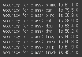
지금까지는 CPU 환경이었는데, 이 neural network를 GPU에서 돌리면 어떻게 될까?
Training on GPU
Tensor를 GPU에 transfer하는 것처럼, neural net을 GPU에 transfer해보자!
먼저 우리가 가진 device가 CUDA를 사용할 수 있는지 살펴보자!
device = torch.device('cuda:0' if torch.cuda.is_available() else 'cpu')

# Assuming that we are on a CUDA machine, this should print a CUDA device:

print(device)
cuda:0
cuda를 사용할 수 있다면 위와 같은 결과가 나온다.
모든 모듈에 가서 parameter와 buffer를 CUDA tensor로 변환해준다.
모든 과정에서 GPU에 input과 target도 전송해야 한다는 것을 잊지 말자!
net.to(device)

inputs, labels = data[0].to(device), data[1].to(device)