[PyTorch] Transfer Learning

참고 사이트

cs231n에서 말하는 전이학습

(무작위 초기화를 통해) 맨 처음부터 합성곱 신경망(Convolutional Network) 전체를 학습하는 사람은 매우 적다. 충분한 크기의 데이터셋을 갖추기는 실제로 드물기 때문이다.
하지만 매우 큰 데이터셋(ex. 100가지 분류에 대해 120만 개의 이미지가 포함된 ImageNet)에서 합성곱 신경망(ConvNet)을 미리 학습한 후, 이 합성곱 신경망을 관심있는 작업의 초기 설정 or 고정된 특징 추출기(fixed feature extractor)로 사용한다.

전이학습 시나리오의 주요한 2가지

• 합성곱 신경망의 미세조정(finetuning)

  • 무작위 초기화 대신, 신경망을 ImageNet 1000 데이터셋 등으로 미리 학습한 신경망으로 초기화한다. 학습의 나머지 과정들은 평상시와 같다.

• 고정된 특징 추출기로써의 합성곱 신경망

  • 마지막에 완전히 연결된 계층을 제외한 모든 신경망의 가중치를 고정한다.
    ➡ 이 마지막의 완전히 연결된 계층은 새로운 무작위의 가중치를 갖는 계층으로 대체되어 이 계층만 학습한다.

---

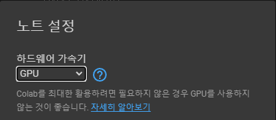
0. 런타임 유형 GPU로 변경하기

colab에서 전이학습을 구현해보자!

먼저 런타임>런타임 유형 변경에서 하드웨어 가속기를 GPU로 변경해줬다.
(CPU로 하면 모델 학습할 때 15~25분이 걸리고, GPU로 하면 1분 정도가 걸리기 때문에 GPU로 하자!)

---

1. Import Modules

# License: BSD
# Author: Sasank Chilamkurthy

from __future__ import print_function, division

import torch
import torch.nn as nn
import torch.optim as optim
from torch.optim import lr_scheduler
import torch.backends.cudnn as cudnn
import numpy as np
import torchvision
from torchvision import datasets, models, transforms
import matplotlib.pyplot as plt
import time
import os
import copy

cudnn.benchmark = True
plt.ion()   # 대화형 모드

--

2. 데이터 불러오기

데이터를 불러오기 위해 torchvision과 torch.utils.data 패키지를 사용한다.

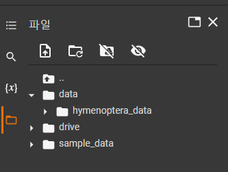
데이터 다운로드 후 data 폴더에 압축 해제를 해준다.

그런데 코드를 실행시키니 아래와 같은 에러가 발생했다.

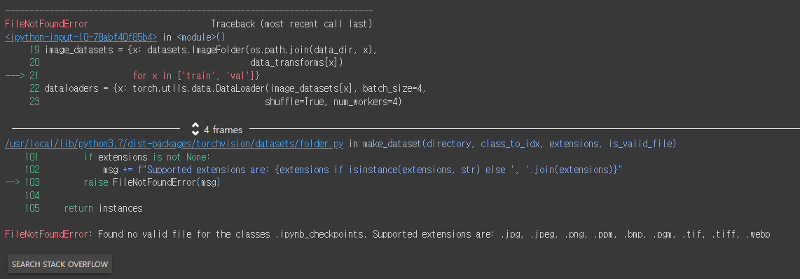
그래서 구글 드라이브에 업로드 후, 파일 아이콘 세 번째에 있는 드라이브 마운트를 해서 경로도 드라이브로 수정해주니 해결되었다.

경로 수정한 코드

# 학습을 위해 데이터 증가(augmentation) 및 일반화(normalization)
# 검증을 위한 일반화
data_transforms = {
    'train': transforms.Compose([
        transforms.RandomResizedCrop(224),
        transforms.RandomHorizontalFlip(),
        transforms.ToTensor(),
        transforms.Normalize([0.485, 0.456, 0.406], [0.229, 0.224, 0.225])
    ]),
    'val': transforms.Compose([
        transforms.Resize(256),
        transforms.CenterCrop(224),
        transforms.ToTensor(),
        transforms.Normalize([0.485, 0.456, 0.406], [0.229, 0.224, 0.225])
    ]),
}

data_dir = 'drive/MyDrive/cs231n/hymenoptera_data'
image_datasets = {x: datasets.ImageFolder(os.path.join(data_dir, x),
                                          data_transforms[x])
                  for x in ['train', 'val']}
dataloaders = {x: torch.utils.data.DataLoader(image_datasets[x], batch_size=4,
                                             shuffle=True, num_workers=4)
              for x in ['train', 'val']}
dataset_sizes = {x: len(image_datasets[x]) for x in ['train', 'val']}
class_names = image_datasets['train'].classes

device = torch.device("cuda:0" if torch.cuda.is_available() else "cpu")

실행시키니까 아래와 같은 결과창이 나온다. Warning이 발생했는데... 일단 넘어가보자.

/usr/local/lib/python3.7/dist-packages/torch/utils/data/dataloader.py:490: UserWarning: This DataLoader will create 4 worker processes in total. Our suggested max number of worker in current system is 2, which is smaller than what this DataLoader is going to create. Please be aware that excessive worker creation might get DataLoader running slow or even freeze, lower the worker number to avoid potential slowness/freeze if necessary.
cpuset_checked))

---

3. 일부 이미지 시각화하기

데이터 증가를 이해하기 위해 일부 학습용 이미지를 시각화해보자.

def imshow(inp, title=None):
    """Imshow for Tensor."""
    inp = inp.numpy().transpose((1, 2, 0))
    mean = np.array([0.485, 0.456, 0.406])
    std = np.array([0.229, 0.224, 0.225])
    inp = std * inp + mean
    inp = np.clip(inp, 0, 1)
    plt.imshow(inp)
    if title is not None:
        plt.title(title)
    plt.pause(0.001)  # 갱신이 될 때까지 잠시 기다립니다.


# 학습 데이터의 배치를 얻습니다.
inputs, classes = next(iter(dataloaders['train']))

# 배치로부터 격자 형태의 이미지를 만듭니다.
out = torchvision.utils.make_grid(inputs)

imshow(out, title=[class_names[x] for x in classes])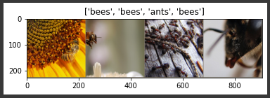

---

4. 모델 학습하기

모델을 학습하기 위한 함수를 작성해보자.
➡ 함수 안에는 학습률 관리(learning rate scheduling)과 최적의 모델을 구하는 내용이 들어간다.

schedule 매개변수: torch.optim.lr_scheduler의 LR 스케쥴러 객체

def train_model(model, criterion, optimizer, scheduler, num_epochs=25):
    since = time.time()

    best_model_wts = copy.deepcopy(model.state_dict())
    best_acc = 0.0

    for epoch in range(num_epochs):
        print(f'Epoch {epoch}/{num_epochs - 1}')
        print('-' * 10)

        # 각 에폭(epoch)은 학습 단계와 검증 단계를 갖습니다.
        for phase in ['train', 'val']:
            if phase == 'train':
                model.train()  # 모델을 학습 모드로 설정
            else:
                model.eval()   # 모델을 평가 모드로 설정

            running_loss = 0.0
            running_corrects = 0

            # 데이터를 반복
            for inputs, labels in dataloaders[phase]:
                inputs = inputs.to(device)
                labels = labels.to(device)

                # 매개변수 경사도를 0으로 설정
                optimizer.zero_grad()

                # 순전파
                # 학습 시에만 연산 기록을 추적
                with torch.set_grad_enabled(phase == 'train'):
                    outputs = model(inputs)
                    _, preds = torch.max(outputs, 1)
                    loss = criterion(outputs, labels)

                    # 학습 단계인 경우 역전파 + 최적화
                    if phase == 'train':
                        loss.backward()
                        optimizer.step()

                # 통계
                running_loss += loss.item() * inputs.size(0)
                running_corrects += torch.sum(preds == labels.data)
            if phase == 'train':
                scheduler.step()

            epoch_loss = running_loss / dataset_sizes[phase]
            epoch_acc = running_corrects.double() / dataset_sizes[phase]

            print(f'{phase} Loss: {epoch_loss:.4f} Acc: {epoch_acc:.4f}')

            # 모델을 깊은 복사(deep copy)함
            if phase == 'val' and epoch_acc > best_acc:
                best_acc = epoch_acc
                best_model_wts = copy.deepcopy(model.state_dict())

        print()

    time_elapsed = time.time() - since
    print(f'Training complete in {time_elapsed // 60:.0f}m {time_elapsed % 60:.0f}s')
    print(f'Best val Acc: {best_acc:4f}')

    # 가장 나은 모델 가중치를 불러옴
    model.load_state_dict(best_model_wts)
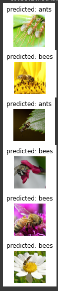
    return model

---

5. 모델 예측값 시각화하기

일부 이미지에 대한 예측값을 보여주는 함수를 작성해보자.

def visualize_model(model, num_images=6):
    was_training = model.training
    model.eval()
    images_so_far = 0
    fig = plt.figure()

    with torch.no_grad():
        for i, (inputs, labels) in enumerate(dataloaders['val']):
            inputs = inputs.to(device)
            labels = labels.to(device)

            outputs = model(inputs)
            _, preds = torch.max(outputs, 1)

            for j in range(inputs.size()[0]):
                images_so_far += 1
                ax = plt.subplot(num_images//2, 2, images_so_far)
                ax.axis('off')
                ax.set_title(f'predicted: {class_names[preds[j]]}')
                imshow(inputs.cpu().data[j])

                if images_so_far == num_images:
                    model.train(mode=was_training)
                    return
        model.train(mode=was_training)

---

6. 합성곱 신경망 미세조정(finetuning)

미리 학습된 모델을 불러온 후, 마지막의 완전히 연결된 계층을 초기화한다.

model_ft = models.resnet18(pretrained=True)
num_ftrs = model_ft.fc.in_features
# 여기서 각 출력 샘플의 크기는 2로 설정합니다.
# 또는, nn.Linear(num_ftrs, len (class_names))로 일반화할 수 있습니다.
model_ft.fc = nn.Linear(num_ftrs, 2)

model_ft = model_ft.to(device)

criterion = nn.CrossEntropyLoss()

# 모든 매개변수들이 최적화되었는지 관찰
optimizer_ft = optim.SGD(model_ft.parameters(), lr=0.001, momentum=0.9)

# 7 에폭마다 0.1씩 학습률 감소
exp_lr_scheduler = lr_scheduler.StepLR(optimizer_ft, step_size=7, gamma=0.1)

학습 및 평가

model_ft = train_model(model_ft, criterion, optimizer_ft, exp_lr_scheduler,
                       num_epochs=25)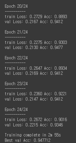

visualize_model(model_ft)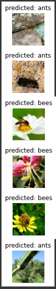

---

7. 고정된 특징 추출기로써의 합성곱 신경망

마지막 계층을 제외한 신경망의 모든 부분을 고정해야 한다.

requires_grad = False로 설정해 매개변수를 고정하여 backward() 중에 경사도가 계산되지 않도록 해야 한다. (참고)

model_conv = torchvision.models.resnet18(pretrained=True)
for param in model_conv.parameters():
    param.requires_grad = False

# 새로 생성된 모듈의 매개변수는 기본값이 requires_grad=True 임
num_ftrs = model_conv.fc.in_features
model_conv.fc = nn.Linear(num_ftrs, 2)

model_conv = model_conv.to(device)

criterion = nn.CrossEntropyLoss()

# 이전과는 다르게 마지막 계층의 매개변수들만 최적화되는지 관찰
optimizer_conv = optim.SGD(model_conv.fc.parameters(), lr=0.001, momentum=0.9)

# 7 에폭마다 0.1씩 학습률 감소
exp_lr_scheduler = lr_scheduler.StepLR(optimizer_conv, step_size=7, gamma=0.1)

학습 및 평가

합성곱 신경망 미세조정과 비교했을 때 약 절반 가량의 시간만 소요된다.
이는 대부분의 신경망에서 경사도를 계산할 필요가 없기 때문이다! 하지만 순전파는 계산이 필요하다.

model_conv = train_model(model_conv, criterion, optimizer_conv,
                         exp_lr_scheduler, num_epochs=25)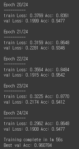

visualize_model(model_conv)

plt.ioff()
plt.show()