코딩테스트 연습
알고리즘
SQL
미니 프로젝트
딥러닝 모델링을 위한 다양한 함수
- 신경망 구성에 필요한 함수들에 대해 알아봅시다!
- 선형 계층(Linear Layer)
- 손실 함수(Loss Function)
- 최적화 함수(Optimizer)
학습 목표
- 딥러닝 구성을 위한 다양한 기능들에 대해서 알 수 있다.
- GPU 활용법 알기
- 선형 계층 구현하기
- 손실함수 구현해보기
- 경사하강법 구현해보기
- 텐서의 연산 진행 내용을 기록하는 기능 배우기
GPU 사용법 알기
- 딥러닝은 연산량이 많기 때문에 GPU를 활용한 병렬 연산이 필요
- Pytorch는 CUDA를 활용하여 GPU 연산을 진행
- GPU, CPU 활용 방법에 대해서 알아보자
import torch

# GPU를 사용하고 싶은 때는 명시적으로 표시!
torch.zeros(2,2, device='cuda')
tensor([[0., 0.],
[0., 0.]], device='cuda:0')- GPU 사용하는 경우
device='cuda:0'이 뒤에 붙음- 코랩 기본 설정은 CPU라 런타임 유형 변경을 하지 않으면 오류 발생
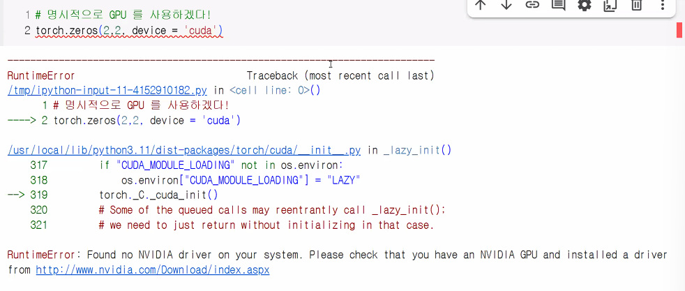
- 코랩 기본 설정은 CPU라 런타임 유형 변경을 하지 않으면 오류 발생
CPU ↔ GPU 데이터 복사
- 제공되는 데이터 세트는 대부분 CPU 환경에서 생성됨
- 훈련 시 GPU로 연산하기 위해 데이터 복사 필요
# CPU에서 데이터 생성(데이터 선언)
t_cpu = torch.LongTensor(2,2)

# GPU로 복사: .cuda
t_gpu = t_cpu.cuda()

# 다시 CPU로 복사(예: GPU에서 학습한 데이터의 결과를 matplotlib 등에서 확인 시 필요)
t_cpu2 = t_gpu.cpu()
선형 계층 구현
- 선형 계층(Linear Layer): 신경망을 구성하는 기본적인 구성 요소
- 퍼셉트론의 '선형 모델' 역할
- 기본 형태
- y = wx + b
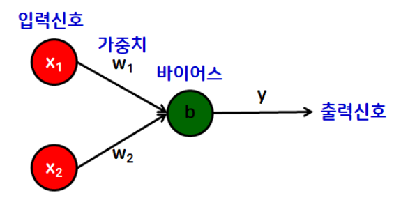
- y = wx + b
torch.nn- 신경망을 구성할 때 사용하는 다양한 기능들이 들어 있는 공간
- 모듈화된 신경망 레이어, 손실 함수, 활성화 함수 등을 포함하고 있음
nn.Linear
# 선형 함수 사용해보기
import torch
import torch.nn as nn # 신경망(neural network)
# 모듈화된 신경망 레이어, 손실 함수, 활성화 함수 등을 포함

# 임의의 입력 데이터 생성
x = torch.randn(4,3) # (샘플 수, 입력 특성 수)

# 선형 함수 생성
# nn.Linear(입력 특성의 수, 출력 특성의 수)
linear = nn.Linear(in_features=3, out_features=2) # 파라미터 적지 않고 넣을 거면 (in, out) 순서로
# 예시를 보여주기 위해 출력 특성의 수를 임의로 2라 정함
# 선형 함수 선언하면 임의의 w, b 값이 생성됨
# in_features: 입력 특성 수, out_features: 출력 특성 수

# 머신러닝 모델 중간층 Dense에 해당
# 중간층 역할이라 in과 out이 모두 있음

y = linear(x)
print("x:", x, sep="\n")
print("\nx의 형태", x.shape, sep="\n")
print("\ny:", y, sep="\n") # 모델이 예측한 결과
print("\ny의 형태", y.size(), sep="\n") # (4,2) → (샘플 수, 출력 특성 수)
x:
tensor([[-0.2281, 1.1929, 1.0563],
[ 0.1469, 1.3057, -2.7503],
[-0.1733, 2.3314, 1.6344],
[-2.0424, -2.4483, 0.7588]])
x의 형태
torch.Size([4, 3])
y:
tensor([[-0.5343, 0.7203],
[-2.0367, 1.1475],
[-0.7623, 1.1586],
[ 0.0985, -0.8951]], grad_fn=<AddmmBackward0>)
y의 형태
torch.Size([4, 2])# linear가 가지고 있는 파라미터(w,b) 확인
print(list(linear.parameters()))
# w, b 순으로 출력
# w → (출력, 입력) 형태로 나옴 → (2,3)
# 아래와 같은 방법도 가능
print(linear.weight)
print(linear.bias)>>>[Parameter containing:
tensor([[ 0.4632, -0.4395, 0.4273],
[ 0.0399, 0.4316, -0.0955]], requires_grad=True), Parameter containing:
tensor([-0.3557, 0.3154], requires_grad=True)]
>>>Parameter containing:
tensor([[ 0.4632, -0.4395, 0.4273],
[ 0.0399, 0.4316, -0.0955]], requires_grad=True)
>>>Parameter containing:
tensor([-0.3557, 0.3154], requires_grad=True)In PyTorch, the shape of the weight matrix for a torch.nn.Linear layer is typically (out_features, in_features).
Example:
If you define a linear layer as nn.Linear(10, 5), the weight matrix associated with this layer will have a shape of (5, 10). This means it has 5 rows (corresponding to out_features) and 10 columns (corresponding to in_features).
Accessing the shape:
You can access the shape of the weight matrix for a specific layer within your model using its weight.shape attribute. For example, if you have a model my_model and a linear layer named fc1 within it, you can get the weight matrix shape by my_model.fc1.weight.shape.
Note on Transpose:
While the weight matrix is stored in (out_features, in_features) shape, PyTorch's F.linear function (which nn.Linear utilizes) performs a matrix multiplication of the input with the transposed weight matrix (input.matmul(weight.t())).
This means that effectively, during the forward pass, the operation is equivalent to multiplying the input with a matrix of shape (in_features, out_features). This design choice is primarily for optimization and historical reasons, and it does not affect the logical interpretation of the weight matrix dimensions.
손실 함수 구현
- loss(손실; 오차)
- 실제값과 예측값의 차이
- 오차가 작을수록 우수한 모델일 가능성이 높다고 판단!
- 대표 손실 함수(loss function)
- 평균제곱오차(MSE)
구현 방법 (3가지)
- 함수를 직접 구현
def mse(y, y_pred):
    loss = ((y-y_pred)**2).mean()
    return loss

# 임의의 값을 통해 함수 사용
y = torch.FloatTensor([[1,2],[3,4]])
y_pred = torch.FloatTensor([[1,3],[2,4]])

print(mse(y,y_pred))
# 출력: tensor(0.5000)- torch에서 제공하는 함수 사용
torch.nn.functional을 사용한 손실 함수:mse_loss
import torch.nn.functional as F

# 파이토치에서 제공하는 손실 함수를 구하는 함수 → mse_loss()
F.mse_loss(y,y_pred)
# 출력: tensor(0.5000)- 클래스 사용
- torch.nn을 활용한 손실 함수
nn.Module클래스 내부에서 선언
- torch.nn을 활용한 손실 함수
import torch.nn as nn

# 객체 생성
mse_loss = nn.MSELoss()

# 사용
mse_loss(y,y_pred)
# 출력: tensor(0.5000)
언제 사용할까?
- mse_loss 함수: 간단한 결과 확인
- nn.MSELoss 클래스: 신경망 구성 시 사용
- 커스터마이징이 가능하다는 장점이 있음
- 1~3번 중 2번과 3번을 주로 사용
- 1번: 함수를 눈으로 보고 싶을 때
- 2번: 단순 확인
- 3번: 신경망 구성 시
경사하강법 구현을 위해 알아야 하는 내용
-
경사하강법(Gradient Descent)
- 손실 함수가 최소가 되는 최적의 파라미터(W,b)를 찾기 위한 최적화 기법
- 최적화 함수 == optimizer라고 부름
-
경사하강법 구현을 위해 '파이토치 오토그래드(AutoGrad) 개념을 알아야 함!
- 해당 개념은 '오차 역전파'와 깊은 관련이 있음
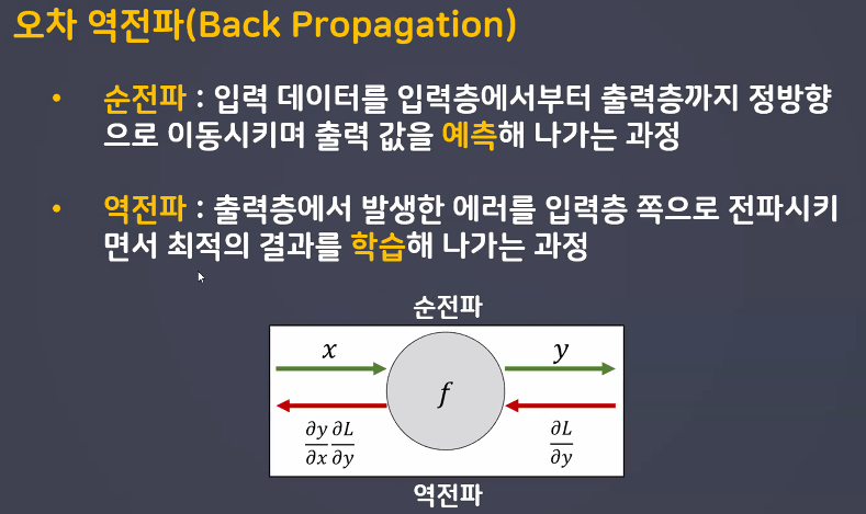
- 전체 process 꼭 이해하기
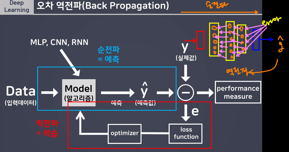
- 해당 개념은 '오차 역전파'와 깊은 관련이 있음
경사하강법 구현을 위해 '파이토치 오토그래드(AutoGrad)' 개념을 알아야 함!
파이토치 오토그래드(AutoGrad)
- torch.autograd → Tensor의 모든 연산에 자동 미분 제공
requireds_grad_(): True 지정 시 해당 텐서에서 이루어지는 모든 연산들을 추척, 기록하기 시작backward(): 추적 기록을 따라 역방향으로 자동 미분을 수행하고 계산된 기울기를 반영 (→ 오차역전파)
# requires_grad_(): 인플레이스 연산(_) → 연산 후 기존 텐서에 값을 덮어씌워 저장하는 연산
x = torch.FloatTensor([[1, 2], [3, 4]]).requires_grad_(True)
print(x)

# 학습 진행
x2 = x ** 2 - 4
print(x2)
y = x2.sum()
print(y)

print(x.grad) # x는 연산을 위한 대상
# backward 전이라 덮어씌워진 적이 없기 때문에 None이 출력됨

y.backward()
print(x.grad) # backward 이후에는 계산된 기울기 값이 반영되어 있음
tensor([[1., 2.],
[3., 4.]], requires_grad=True)
tensor([[-3., 0.],
[ 5., 12.]], grad_fn=<SubBackward0>)
tensor(14., grad_fn=<SumBackward0>)
None
tensor([[2., 4.],
[6., 8.]])- 임의의 텐서를 생성하여 requires_grad 개념 알기
a = torch.randn(3,3)
a += 3 # a = a + 3

print(a)
print(a.requires_grad) # 누적해달라고 안 했으니까 False

a.requires_grad_(True) # requires_grad = True → 인플레이스 연산
print(a.requires_grad)

b = (a*a).sum()
print(b) # sum 연산 수행이 기록
print(b.requires_grad)
tensor([[3.3033, 2.3428, 1.7929],
[1.9171, 1.4089, 2.6518],
[5.2463, 2.3058, 1.7487]])
False
True
b = (a*a).sum()
print(b) # sum 연산 수행이 기록
print(b.requires_grad)
tensor(68.2057, grad_fn=<SumBackward0>)
True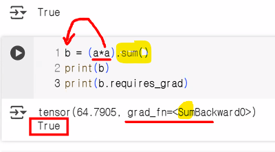
→ 마지막 연산이 sum이어서 SumBackward
x = torch.ones(3,3,requires_grad=True)
print(x)

y = x+5
print(y)
# 더하기 연산 기록

z = y*y

# 중간 텐서에서 grad를 확인하고 싶다면?
y.retain_grad()
z.retain_grad()

out = z.mean()
print(z,out,sep="\n")
tensor([[1., 1., 1.],
[1., 1., 1.],
[1., 1., 1.]], requires_grad=True)
tensor([[6., 6., 6.],
[6., 6., 6.],
[6., 6., 6.]], grad_fn=<AddBackward0>)
tensor([[36., 36., 36.],
[36., 36., 36.],
[36., 36., 36.]], grad_fn=<MulBackward0>)
tensor(36., grad_fn=<MeanBackward0>)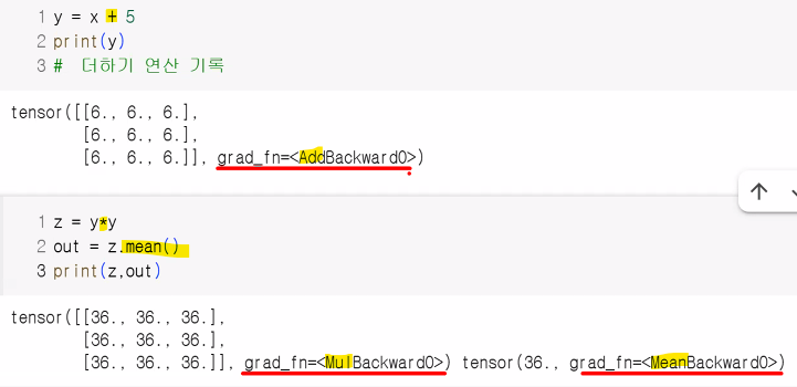
- 순전파 계산 완료 후 backward() 호출하면 자동으로 역전파 계산이 되며, grad 속성에 누적됨
print(out)
out.backward()
print(out.grad) # leaf Tensor(연산 시작점, 첫 텐서)가 아니면 grad 확인 불가

# 기본 설정으로 되어 있으면
# leaf Tensor가 아닌 grad는 확인할 수 없음
# 중간의 텐서에서도 grad를 확인하고 싶다면
# retain_grad() 사용!

# 가장 초기의 x에서만 grad를 확인할 수 있다
print(x.grad)

print(z.grad)
# retain_grad() 사용했기 때문에 확인 가능
>>> tensor(36., grad_fn=<MeanBackward0>)
>>> UserWarning: The .grad attribute of a Tensor that is not a leaf Tensor is being accessed.
Its .grad attribute won't be populated during autograd.backward().
If you indeed want the .grad field to be populated for a non-leaf Tensor,
use .retain_grad() on the non-leaf Tensor.
If you access the non-leaf Tensor by mistake, make sure you access the leaf Tensor instead.
>>> tensor([[1.3333, 1.3333, 1.3333],
[1.3333, 1.3333, 1.3333],
[1.3333, 1.3333, 1.3333]])
>>> tensor([[0.1111, 0.1111, 0.1111],
[0.1111, 0.1111, 0.1111],
[0.1111, 0.1111, 0.1111]])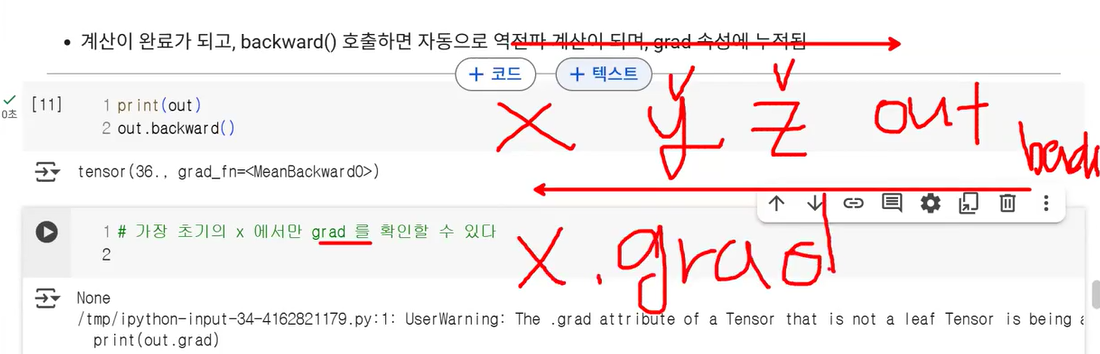
requires_grad_: 어떤 연산을 했는지에 대한 기록(연산 과정에 대한 기록) 덧씌우기
inplace: 연산의 결과에 대한 내용(연산의 결과값을 원본/변수에 덧씌우기)
detach() 함수
- 내용물은 같지만 requires_grad 기록이 다른 완전 새로운 Tensor를 가져올 때 사용
- 연산 그래프에서 분리해 gradient 추적을 멈추는 용도
- 연산 기록이 작성되어 있는 데이터를 기울기 계산에서 배제하고 싶을 때 →
detach()를 쓰면 됨- 결과를 시각화할 때 텐서 연산의 결과를 초기화 후 넘파이 배열로 변경하여 시각화 하는 것이 안전
- 텐서를 끊고(.detach()) 넘파이로 바꿈(.numpy())
- 결과를 시각화할 때 텐서 연산의 결과를 초기화 후 넘파이 배열로 변경하여 시각화 하는 것이 안전
- 메모리를 공유하기 때문에 복사한 텐서의 값을 바꾸면 원본 텐서에도 동일하게 적용
- detach()는 원본 텐서와 메모리를 공유하면서 새로운 텐서를 만듦
- 즉, 새 메모리에 복사(deepcopy)하는 것이 아니라, 원래 텐서의 데이터를 그대로 가리키는 얕은 복사(shallow copy) 형태!
- 이로 인해 detach()로 만든 텐서에 in-place 연산(예: 값 변경, zero(), add() 등)을 하면, 원본 텐서의 값도 같이 변경됨
- detach()는 원본 텐서와 메모리를 공유하면서 새로운 텐서를 만듦
import torch

x = torch.tensor([1., 2., 3.], requires_grad=True)
y = x.detach()
y[0] = 100
print(x)  # tensor([100., 2., 3.], requires_grad=True)
print(y)  # tensor([100., 2., 3.])
이런 일이 일어나는 이유는 x와 y가 같은 메모리 공간을 공유하기 때문입니다. 즉, y를 바꾸면 x도 바뀌고, 그 반대도 가능합니다.
이와 달리, clone() 함수는 완전히 새로운 메모리에 데이터를 복사하기 때문에, clone()으로 생성한 텐서의 값을 변경하더라도 원본 텐서에는 영향을 주지 않습니다.
정리:
detach() 텐서는 원본과 메모리를 공유하므로, 한 쪽에서 값을 바꾸면 다른 쪽도 바뀐다.
clone() 텐서는 메모리를 새로 할당받기 때문에 한 쪽을 바꿔도 서로 영향 없다.
이런 동작 덕분에 detach()로 생성한 텐서를 신경 쓸 때는 in-place 연산에 특히 주의해야 하며, 원본 데이터를 정말 독립적으로 쓰려면 clone().detach() 혹은 detach().clone()처럼 둘 다 써서 완전히 분리하는 것이 안전합니다.
detach()는 텐서를 연산 그래프에서 분리해서 이후 연산에서 gradient가 계산되지 않도록 해준다.
즉, 기존 텐서와 같은 데이터를 가지지만, 분리된 새로운 텐서를 만들어 gradient 추적을 멈춘다.
- 동작 및 역할
- 연산 기록과의 분리
- detach() 함수는 해당 텐서를 현재까지의 연산 그래프(Computational Graph) 에서 분리해, 이후의 계산에서 자동 미분(autograd)이 추적하지 않게 만듭니다. 즉, 분리된 텐서는 그 이후 연산에 대해 gradient가 계산되지 않습니다.
- requires_grad 값과의 관계
- detach()가 반환하는 새 텐서는 requires_grad=False가 되며, 따라서 그 텐서를 기반으로 추가 연산을 하더라도 gradient 기록이 되지 않습니다. 하지만 본래의 텐서는 변하지 않고, detach()는 연산 기록만 끊어주는 역할입니다. (연산 그래프와 분리하여 gradient 추적을 멈춤)
- 실제 사용 목적
- 연산 그래프 일부에서 gradient 흐름을 끊고 싶을 때 (예: GAN 등에서 generator의 값을 discriminator에 넣으면서 gradient 전달을 막고 싶을 때)
- 학습 중간 결과를 복사하거나, 연산 기록 없이 numpy 등으로 데이터를 변환할 때
- 메모리 사용량 절감 등 목적에서 중간 텐서의 gradient 추적을 중단할 때
- 연산 기록과의 분리
- 텐서는 연산 그래프를 따라 연산 결과(데이터)와 연산 기록을 모두 가집니다. 하지만, detach를 사용하면 해당 텐서와 동일한 값을 가지되, 연산 그래프와 연결이 끊어진 새 텐서를 얻어 이후 계산에서 gradient가 추적되지 않도록 할 수 있습니다.
out.requires_grad
out2 = out.detach()
print(out.requires_grad)
print(out2.requires_grad)
print(out)
print(out2)
True
False
tensor(36., grad_fn=<MeanBackward0>)
tensor(36.)자동 미분 흐름 예제
- 실제 미분값이 어떻게 흐르는지 봐보자
- 계산 흐름:
backward()를 통해 을 계산하면 값이a.grad에 채워짐
a = torch.ones(2, 2, requires_grad=True)
print(a)

# 연산 전, 후 비교를 위해 a 데이터의 정보 출력
print(a.data)
print(a.grad)
print(a.grad_fn)

# 현재 상태에서는 아무 연산이 안 됐기 때문에 None 값이 출력

b = a+2
print(b)

c = b**2
print(c)

out = c.sum()
print(out)

# 오차역전파
out.backward()

print(a.data)
print(a.grad)
print(a.grad_fn)

print(b.data)
print(b.grad) # 중간 텐서에서는 grad를 확인할 수 없다
print(b.grad_fn)
# grad_fn: 현재 텐서가 연산을 통해 결과값이 만들어졌는지에 대한 기록
tensor([[1., 1.],
[1., 1.]], requires_grad=True)
tensor([[1., 1.],
[1., 1.]])
None
None
tensor([[3., 3.],
[3., 3.]], grad_fn=<AddBackward0>)
tensor([[9., 9.],
[9., 9.]], grad_fn=<PowBackward0>)
tensor(36., grad_fn=<SumBackward0>)
tensor([[1., 1.],
[1., 1.]])
tensor([[6., 6.],
[6., 6.]])
None
tensor([[3., 3.],
[3., 3.]])
>>> None
>>> <AddBackward0 object at 0x78908ed42d40>
>>> UserWarning: The .grad attribute of a Tensor that is not a leaf Tensor is being accessed. | 속성/함수 | 설명 |
|---|---|
.grad | 역전파로 계산된 기울기(gradient) 값 |
.grad_fn | 현재 텐서가 어떤 연산의 결과인지 추적하는 함수 |
requires_grad | 이 텐서의 미분값을 추적할지 여부 설정(True/False) |
.detach() | 현재 텐서를 계산 그래프에서 분리한 복사본 생성 (미분 추적 안함) |
경사하강법 구현
import torch
import torch.nn.functional as F

# 정답 데이터 (목표 텐서)
t = torch.FloatTensor([[0.1, 0.2, 0.3],
                       [0.4, 0.5, 0.6],
                       [0.7, 0.8, 0.9]])
print(t)
# 임의의 텐서 (목표 텐서와 동일한 크기를 갖는 랜덤 텐서 생성)
x = torch.rand_like(t).requires_grad_(True)
print(x)

# 우리의 목표: x를 t에 가까워지게 할 예정
# 랜덤 텐서가 목표 텐서와의 오차를 구해서 기준보다 작아질 때까지 연산 진행
th = 1e-5 # 부동소수점(0.00001)
learning_rate = 1.0 # 학습률
epochs = 0 # 초기 반복횟수 초기화

# 학습 전 목표 텐서(t), 랜덤 텐서(x) 손실값 계산
loss = F.mse_loss(x,t)

# 경사하강법
while loss>th: # loss가 th 보다 크면 반복
    epochs += 1
    # 오차역전파
    loss.backward()

    # 랜덤 텐서 값 업데이트 (경사하강법 공식 적용)
    x = x - learning_rate*x.grad

    # 텐서 해제(detach)
    x.detach_() # 안 해주면 현재가지의 연산 기록이 다음 epoch에도 누적됨
    # 반드시 인플레이스 함수 사용할 것! (변화를 계속 x에 덮어씌워야 함)
    x.requires_grad_(True)

    # 변화 후 오차 확인
    loss = F.mse_loss(x,t)

    # 출력(오차, 현재 x)
    print(f"{epochs} epoch, Loss: {loss:.4e}")
    print(x)
tensor([[0.1000, 0.2000, 0.3000],
[0.4000, 0.5000, 0.6000],
[0.7000, 0.8000, 0.9000]])
tensor([[0.5597, 0.5974, 0.8898],
[0.3020, 0.7925, 0.6637],
[0.0954, 0.8635, 0.2824]], requires_grad=True)
1 epoch, Loss: 1.0535e-01
tensor([[0.4576, 0.5091, 0.7587],
[0.3238, 0.7275, 0.6496],
[0.2298, 0.8494, 0.4196]], requires_grad=True)
2 epoch, Loss: 6.3733e-02
tensor([[0.3781, 0.4404, 0.6568],
[0.3407, 0.6770, 0.6386],
[0.3343, 0.8384, 0.5264]], requires_grad=True)
3 epoch, Loss: 3.8554e-02
tensor([[0.3163, 0.3870, 0.5775],
[0.3539, 0.6376, 0.6300],
[0.4155, 0.8299, 0.6094]], requires_grad=True)
4 epoch, Loss: 2.3323e-02
tensor([[0.2682, 0.3454, 0.5158],
[0.3641, 0.6071, 0.6233],
[0.4788, 0.8233, 0.6740]], requires_grad=True)
5 epoch, Loss: 1.4109e-02
tensor([[0.2309, 0.3131, 0.4679],
[0.3721, 0.5833, 0.6181],
[0.5279, 0.8181, 0.7242]], requires_grad=True)
6 epoch, Loss: 8.5351e-03
tensor([[0.2018, 0.2880, 0.4306],
[0.3783, 0.5648, 0.6141],
[0.5662, 0.8141, 0.7633]], requires_grad=True)
7 epoch, Loss: 5.1632e-03
tensor([[0.1792, 0.2684, 0.4016],
[0.3831, 0.5504, 0.6110],
[0.5959, 0.8109, 0.7937]], requires_grad=True)
8 epoch, Loss: 3.1234e-03
tensor([[0.1616, 0.2532, 0.3790],
[0.3869, 0.5392, 0.6085],
[0.6190, 0.8085, 0.8173]], requires_grad=True)
9 epoch, Loss: 1.8895e-03
tensor([[0.1479, 0.2414, 0.3614],
[0.3898, 0.5305, 0.6066],
[0.6370, 0.8066, 0.8357]], requires_grad=True)
10 epoch, Loss: 1.1430e-03
tensor([[0.1372, 0.2322, 0.3478],
[0.3921, 0.5237, 0.6052],
[0.6510, 0.8051, 0.8500]], requires_grad=True)
11 epoch, Loss: 6.9145e-04
tensor([[0.1290, 0.2250, 0.3372],
[0.3938, 0.5184, 0.6040],
[0.6619, 0.8040, 0.8611]], requires_grad=True)
12 epoch, Loss: 4.1829e-04
tensor([[0.1225, 0.2195, 0.3289],
[0.3952, 0.5143, 0.6031],
[0.6704, 0.8031, 0.8697]], requires_grad=True)
13 epoch, Loss: 2.5304e-04
tensor([[0.1175, 0.2151, 0.3225],
[0.3963, 0.5112, 0.6024],
[0.6770, 0.8024, 0.8765]], requires_grad=True)
14 epoch, Loss: 1.5307e-04
tensor([[0.1136, 0.2118, 0.3175],
[0.3971, 0.5087, 0.6019],
[0.6821, 0.8019, 0.8817]], requires_grad=True)
15 epoch, Loss: 9.2599e-05
tensor([[0.1106, 0.2092, 0.3136],
[0.3977, 0.5067, 0.6015],
[0.6861, 0.8015, 0.8858]], requires_grad=True)
16 epoch, Loss: 5.6017e-05
tensor([[0.1082, 0.2071, 0.3106],
[0.3982, 0.5052, 0.6011],
[0.6892, 0.8011, 0.8889]], requires_grad=True)
17 epoch, Loss: 3.3887e-05
tensor([[0.1064, 0.2055, 0.3082],
[0.3986, 0.5041, 0.6009],
[0.6916, 0.8009, 0.8914]], requires_grad=True)
18 epoch, Loss: 2.0499e-05
tensor([[0.1050, 0.2043, 0.3064],
[0.3989, 0.5032, 0.6007],
[0.6934, 0.8007, 0.8933]], requires_grad=True)
19 epoch, Loss: 1.2401e-05
tensor([[0.1039, 0.2034, 0.3050],
[0.3992, 0.5025, 0.6005],
[0.6949, 0.8005, 0.8948]], requires_grad=True)
20 epoch, Loss: 7.5018e-06
tensor([[0.1030, 0.2026, 0.3039],
[0.3994, 0.5019, 0.6004],
[0.6960, 0.8004, 0.8959]], requires_grad=True)실습: 딥러닝 회귀 모델
학습 목표
- 당뇨병 데이터를 활용하여 당뇨 진행도를 파악할 수 있다.
- 데이터 불러오기 → sklearn 제공 데이터
- 입력특성: 443명을 대상으로 당뇨병 환자를 검사한 결과
- 정답 데이터: 1년 뒤 측정한 당뇨병 진행률
import numpy as np
import pandas as pd
import matplotlib.pyplot as plt
import seaborn as sns

from sklearn.datasets import load_diabetes
data = load_diabetes() # 번치 객체

# 데이터프레임에 담기
df_data = pd.DataFrame(data.data, columns=data.feature_names)
df_data['target'] = data.target- 입력 특성 데이터 확인
- age: 나이
- sex: 성별
- bmi: bmi 지수
- bp: 평균 혈압
- s1 ~ s6: 6가지 종류의 혈액 검사 결과 수치
- 정답 데이터
- target: 당뇨 진행률
- 연속형 데이터 → 회귀
- target: 당뇨 진행률
df_data.hist(bins=50, figsize=(15, 10))
plt.show()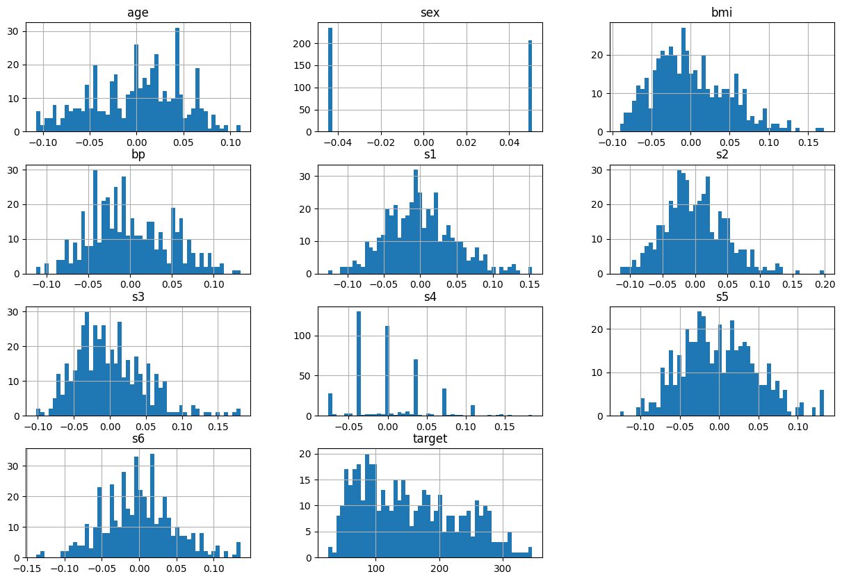
- 문제와 정답으로 분리
# Series, DataFrame은 넘파이 ndarray임 → Tensor로 변경해 주어야 함

# numpy → tensor 변환
import torch
data = torch.tensor(df_data.values).float()

# 문제, 정답 분리
# 10개 → 입력 특성, 1개 → 정답
X=data[:, :-1]
y=data[:, -1]
print(X.shape, y.shape, sep="\n")

# y를 2차원으로 변경
y = y.unsqueeze(1)
y.shape
torch.Size([442, 10])
torch.Size([442])
torch.Size([442, 1])모델 구조 설계: 선형 회귀 모델
import torch.nn as nn

# 선형 회귀 모델 생성
# nn.Linear(in_features=10, out_features=1)
model = nn.Linear(in_features=X.size(-1), out_features=y.size(-1)) # 마지막 차원의 수

# 최적화 함수 생성
import torch.optim as optim

# 모델의 파라미터 값들을 넣어줘야 한다 (w,b)
optimizer = optim.SGD(model.parameters(), lr=0.0001)

# 모델 학습
import torch.nn.functional as F
from tqdm import tqdm # 반복문 진행 시 진행 상황을 시각적으로 보여 주는 로딩 바

epochs = 200000 # 학습 횟수
print_interval = 20000 # 학습 결과 출력을 위한 분리

for i in tqdm(range(epochs)):
    # 모델 적용
    y_pred = model(X)
    # 오차 계산
    loss = F.mse_loss(y_pred, y)

    # 최적화 함수 초기화
    optimizer.zero_grad() # 이전에 반복 계산된 결과 초기화

    # 오차 역전파
    loss.backward()

    # 역전파 단계에서 계산된 기울기로 가중치 업데이트 (w,b)
    optimizer.step()

    if (i+1)%print_interval == 0: # 20만 번의 학습 중 2만 번마다 출력
        print(f"epoch:{i+1}, loss:{loss:.4e}")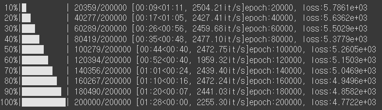
하루 돌아보기
👍 잘한 점
- Autograd, nn.Linear, 경사하강법 추가 공부 진행
- 야간자율학습 참여
- 미니프로젝트 진행
👎 아쉬웠던 점
- 비가 너무 많이 오고 천둥도 치고 그래서 수업 흐름이 자꾸 깨졌음
🔬 개선점
- 외부 자극에도 흔들리지 않는 집중력 기르기