Python 다중 할당 동작 방식

• 다중 할당(Multiple Assignment)

  • 2개 이상의 값을 2개 이상의 변수에 동시에 할당하는 것

    a,b = 1,2
    
    print(a) # 1
    print(b) # 2

    • a와 b 변수 각각의 값을 1, 2로 할당

• 좀 더 복잡한 경우를 생각해보자

  • SingleLinkedList 클래스를 만들어 s3 → s2 → s1 → None 구조를 가지도록 설정

class SingleLinkedList:
    def __init__(self, name, val=0, next=None) -> None:
        self.name = name
        self.val = val
        self.next = next
    def __repr__(self):
        return self.name

s1 = SingleLinkedList(name='s1', val=1)
s2 = SingleLinkedList(name='s2', val=2, next=s1)
s3 = SingleLinkedList(name='s3', val=3, next=s2)

• 여기서 아래와 같은 코드를 실행하면 어떻게 될까?

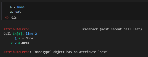
a = None
a.next

→ a는 None으로 초기화가 되어 있고 당연히 a.next를 하게 되면 에러가 난다!

• 하지만 아래와 같이 다중 할당을 하게 되면 a에 SingleLinkedList 객체인 s1이 들어가게 되면서(정확하게는 변수 a가 s1 객체가 참조하고 있는 SingleLinkedList 객체를 참조하게 됨) s1.next를 사용할 수 있음
  • a.next에 s3가 할당되면서 s1의 next가 s3의 객체를 바인딩하게 됨
    • s3 → s2 → s1 → s3

a = None
a, a.next = s1, s3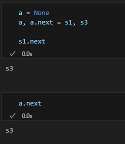

• 더 확실한 이해를 위한 예시
  • 아래 코드를 실행하게 되면 a의 값에는 어떤 값이 들어가게 될까?

a = None
a, a.next, a = s1, s3, a

정답은 None
1. a가 None으로 초기화
2. 기존 s1, s3, a 값은 각각 s1, s3, None으로 초기화되어 있음
3. a = s1, a.next = s3, a=a 순서대로 실행됨
4. a에 s1의 객체가 바인딩되고 a.next에 s3의 객체가 바인딩되고, a에 None이 바인딩됨
5. 앞의 두 할당 작업이 끝나고 a에는 기존 값이던 None이 들어가게 됨
🡆 = 오른쪽 값에 기존 값을 가지고 있고, 왼쪽에 차례대로 값을 바인딩하는 것!

• 마지막 예시

a = None
a, a.next, a, a.next = s1, s3, a, s2

실행하면 오류 발생
🡆 3번째 a에 None값이 들어가기 때문에 a.next는 None.next가 되어 에러

주성분 분석(PCA)

• PCA(Principal Component Analysis)
  • dimensionality reduction(차원 축소)애 쓰이는 대표적인 기법 → 머신러닝, 데이터마이닝, 통계 분석, 노이즈 제거 등 다양한 분야에서 널리 쓰임
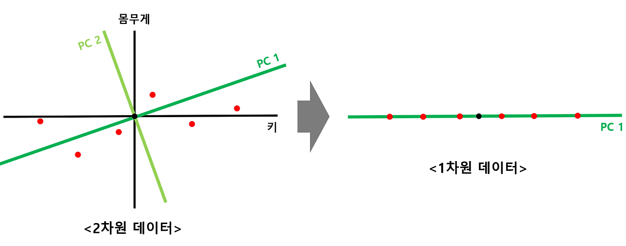
  • 고차원의 데이터를 낮은 차원의 데이터로 바꿔줄 수 있음 → "어떻게 차원을 잘 낮출 것인가?"

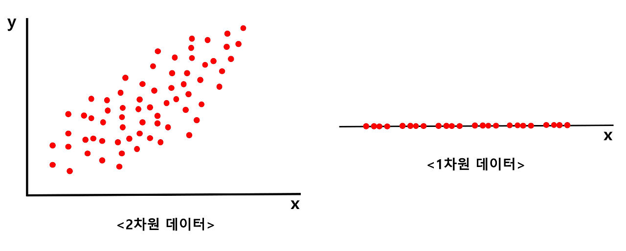
• 왼쪽에 있는 2차원 데이터를 오른쪽에 있는 1차원 데이터로 바꾼다고 생각
  • 아무리 잘 바꾼다고 하더라도 2차원 데이터의 특징을 모두 살리면서 1차원의 데이터로 바꿔줄 수는 없음
  • 차선책으로 최대한 특징을 살리며 차원을 낮춰주는 방법을 고안 → 그 중 하나가 PCA

PCA 과정
(1) N차원의 데이터로부터 Covariance matrix를 생성한다.
(2) 생성된 covariance matrix에서 N개의 Eigenvector, Eigenvalue를 찾는다.
(3) 찾은 Eigenvector를 Eigenvalue가 큰 순서대로 정렬한다.
(4) 줄이기 원하는 차원 개수만큼의 Eigenvector만 남기고 나머지는 쳐낸다.
(5) 남은 Eigenvector를 축으로 하여, 데이터의 차원을 줄인다.

PCA 알고리즘의 직관적 해석

1. 각 축에 대한 평균값을 구한 뒤 해당 점이 원점이 되도록 shift
   
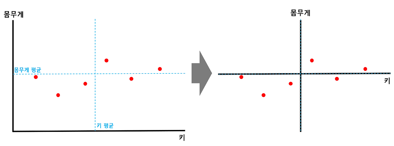
   • x축, y축에 대한 평균값을 구해준 뒤 각 평균값에 해당하는 점들의 교차점이 원점이 되도록 전체 데이터를 shift해줌
2. 데이터에서 원점을 지나는 직선에 수선의 발을 내려 해당 길이가 최대가 되는 직선 찾기
   
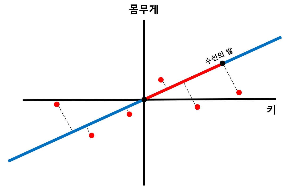
   • 모든 데이터에서 원점을 지나는 직선에 수선의 발을 내리면 원점으로부터 수선의 발까지의 길이를 구할 수 있음
   • 원점을 지나는 직선의 기울기가 변함에 따라 선의 길이 또한 변하게 됨
     • PCA에서는 수선의 발과 원점 사이의 거리 제곱의 합이 최대가 되는 직선을 찾음
     • SS(Sum of Squares): 원점으로부터 수선의 발까지의 길이합

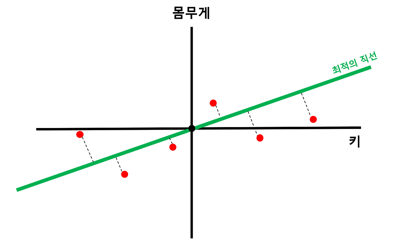
3. 찾은 직선을 PC1으로 설정하고 loading score 구하기
   

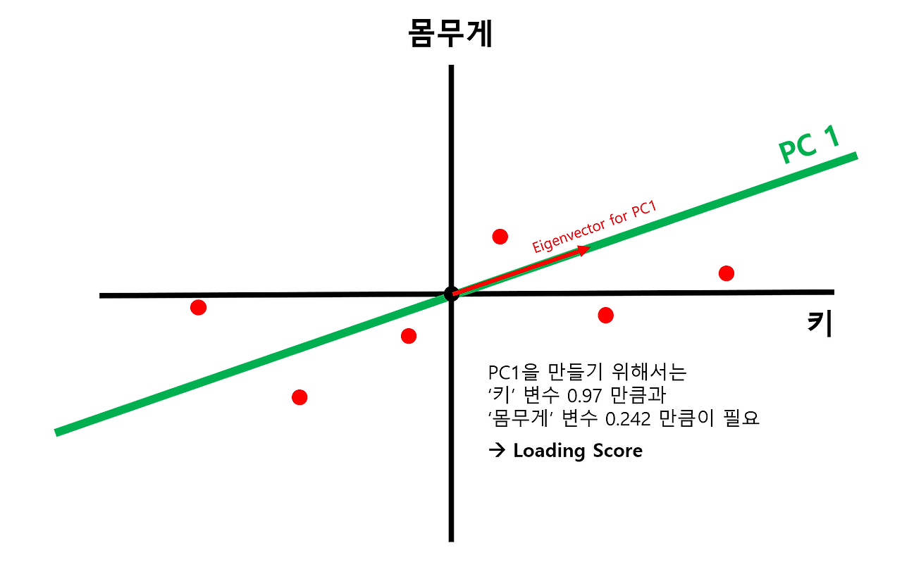
• PC1과 방향이 같은 벡터를 "PC1의 Singular vector" 또는 "PC1의 Eigenvector"라 함
• PC1의 Singular vector의 x축 길이와 y축 길이의 비율을 Loading score라고 함

4. PC1에 직교하는 직선을 PC2로 잡기
   

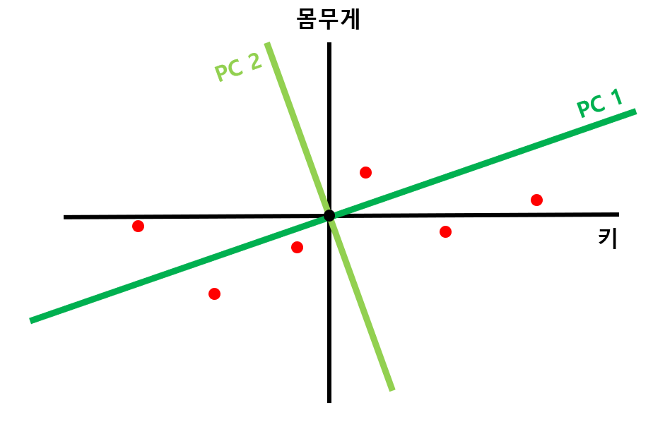
   • 예시의 경우 2차원이므로 PC1에 직교하는 직선이 유일하지만 3차원의 경우라면 PC1에 직교하는 직선이 평면으로 나올 것 → PC1에 직교하는 평면 중 2의 과정을 다시 거쳐 수선의 발까지의 거리 합이 최대가 되는 직선을 선택
   • N차원 데이터에는 N개의 PC 직선이 나온다!

5. PC1과 PC2를 축으로 하여 회전시킨 뒤 scree plot 생성
   

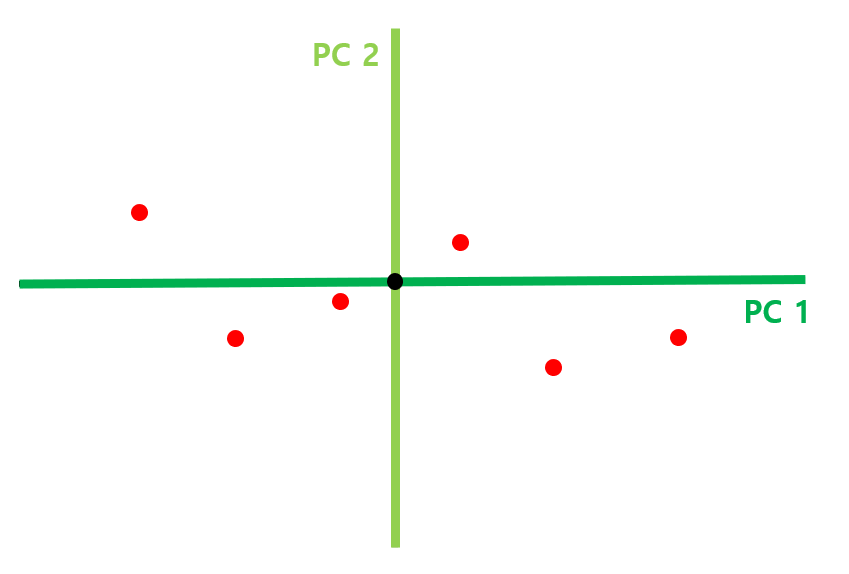
   • scree plot
     • 각 PC 축이 전체 데이터를 얼마나 잘 표현하고 있는지를 나타냄
   • scree plot을 생성하기 위해 PC1과 PC2의 SS 비율을 구해야 함
     
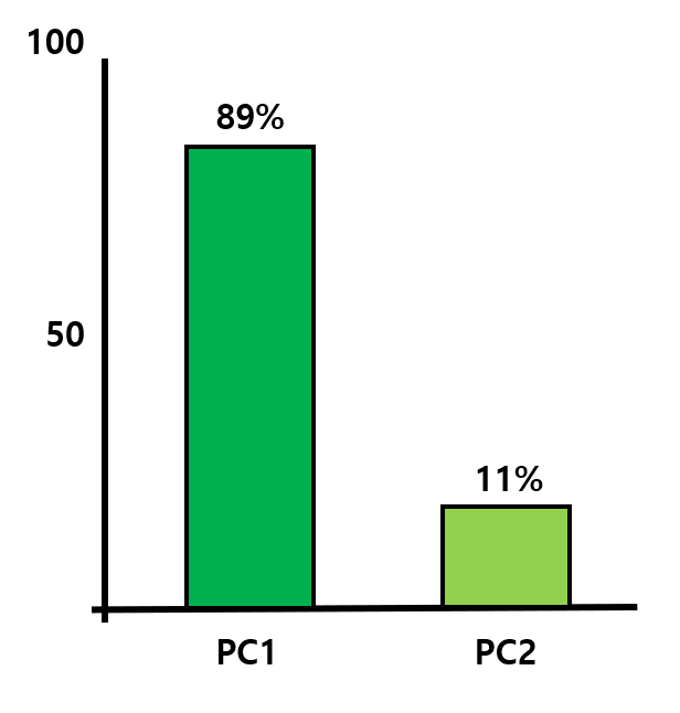
     → PC1 축이 전체 데이터 특징의 89% 정도를 나타내고 있으며, PC2 축이 전체 데이터 특징의 11% 정도를 나타내고 있다는 뜻
     🡆 만약 89% 정도의 특징만으로도 해당 데이터를 잘 나타낼 수 있을 것이라고 판단되면, PC2 축을 제거하고 PC1 축만을 가지고 1차원으로 나타낼 수 있음 → 2차원의 데이터를 1차원으로 바꿈

3차원 데이터가 있는데, PCA를 통해 PC1 PC2 PC3 3개의 축을 잡았고, scree plot 을 그려본 결과 PC1이 73%, PC2가 17%, PC3가 10% 를 차지한다고 해보자. 이러면 개발자에게는 차원을 줄이는 두가지 선택권이 있는 것이다.
(1) 데이터 특징의 90% 를 살리며 3차원에서 2차원으로 차원을 축소하는 선택권 (PC1, PC2 선택)
(2) 데이터 특징의 73% 를 살리며 3차원에서 1차원으로 차원을 축소하는 선택권 (PC1만 선택)
무엇을 선택할지는 현재 시스템의 리소스 상황을 고려하며 선택하면 된다.

PCA 알고리즘의 수학적 해석

1. 고차원의 데이터의 covariance matrix를 구한다.
2. 구한 covariance matrix에서 Eigenstuff(Eigenvector, Eignevalue)를 구한다.
3. 구한 Eigenstuff를 Eigenvalue가 큰것부터 작은 순서대로 정렬한다.
   → 직관적인 해석에서 알아보았던 PC1, PC2, ... 축들이 바로 Eigenvector들이다!
   → 직관적인 해석에서 알아보았던 scree plot에서 각 PC들이 가졌던 비율들이 바로 Eigenvalue값들의 비율이다!
   🡆 즉, Eigenvalue가 큰 것부터 작은 순서대로 정렬한 것이 일종의 scree plot을 그린 것
4. 원하는 만큼 Eigenvector를 쳐냄으로써 차원 축소를 해준다. → Eigenstuff 쳐내기
   
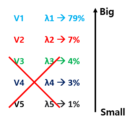
   : 5차원 데이터에서 Eigenstuff를 구한 뒤, Eigenvalue를 기준으로 정렬했다고 해보자. 여기서 만약 내가 5차원 데이터를 2차원으로 줄이겠다! 라고 한다면, Eigenvalue가 큰 두 개를 빼고 나머지 3개를 쳐내면 된다. 그러면 두 개의 Eigenvector를 축으로 하는 2차원 데이터로 차원을 줄일 수 있으며, 해당 2차원 데이터가 나타내는 데이터의 특징은, 두 Eigenvector v1, v2 의 Eigenvalue가 가지는 비율인 86%가 된다.

Variance(분산)

• '데이터가 얼마나 넓게 퍼져있는가'
• 편차의 제곱합의 평균

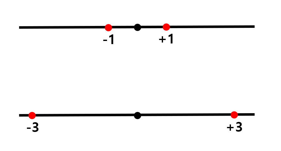
→ 위 데이터의 variance는 (1+0+1)/3 = 2/3, 아래 데이터의 variance는 (9+0+9)/3 = 6

covariance

• 고차원에서의 데이터들 간의 variance를 나타내는 값

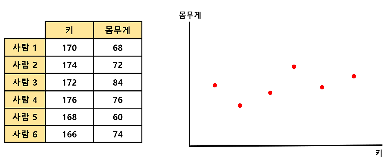
  • 2차원 데이터에서의 분산은 어떻게 구할까?
    • "x축에서의 variance와 y축에서의 variance를 융합하면 된다"
  • 어떻게 두 variance를 융합해야 하나?
    
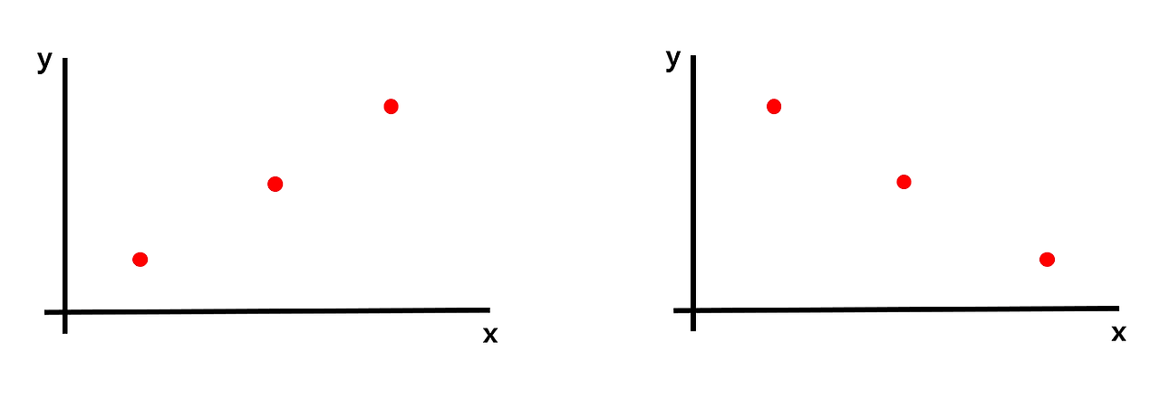
    → 오른쪽과 왼쪽의 데이터의 x축에서의 variance와 y축에서의 variance는 모두 같을 것이므로 단순히 두 variance를 더한 값도 같을 것이다. 하지만 위의 두 데이터는 완전히 다른 분포를 나타내는 데이터이지만, covariance가 같아지므로, 단순히 더하는 방법은 옳지 않은 방법이다.

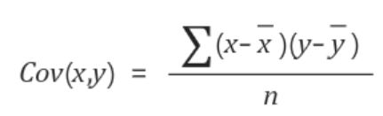
• x값과 y값을 각각 x, y값의 평균의 차 곱하여 더하고(= 내적) n으로 나눠줌으로써 구할 수 있다.
  

• 왼쪽 데이터의 x값과 y값을 곱하면 각각 +4, 0, +4가 된다. 그리고 이 값들을 모두 더해 데이터개수로 나눠주면 covariance가 된다.
• 즉, 왼쪽 데이터의 covariance는 (+4+0+4)/3 = +8/3 이고, 오른쪽 데이터의 covariance는 (-4+0-4)/3 = -8/3이다.

※ 참고 ※
covariance를 구하기 위해 내적하는 과정은 데이터의 평균값이 0 일때만 유효하다. 2차원 데이터일 경우, 데이터의 x축 평균과 y축 평균이 모두 0이어야 하며, 0이 아닐 경우 각각 평균값을 빼주면 된다.

covariance matrix

• covariacne 값을 통해 covariance matrix 라는 행렬을 만들어 낼 수 있다.
• 시그마 기호로 표현하는 2차원 데이터에서의 covariance matrix의 정의는 다음과 같다.
  
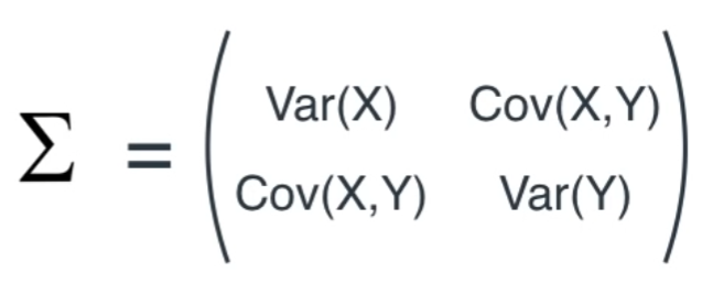
  → 행렬의 주대각선은 각 변수의 variance를 나타내며, i행 j열 데이터는 i와 j 변수의 covariance를 나타낸다.
  물론 i와 j 변수의 covariance와, j와 i 변수의 covariance 는 같으므로 covariance matrix는 주대각선을 축으로 대칭인 symmetric 한 형태가 될 것이다.

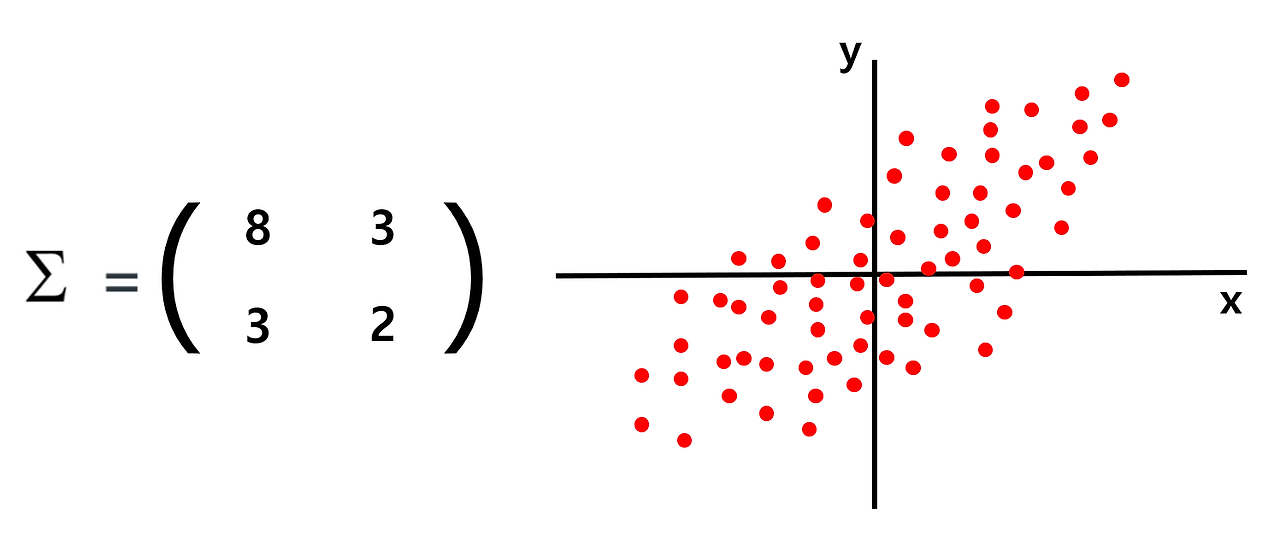
: x의 variance는 y의 variance보다 크므로 데이터는 가로로 길쭉한 형태가 될 것이며, x와 y의 covariance가 양수이므로 1, 3 사분면을 지나는 오른쪽 그림과 같은 형태가 된다.

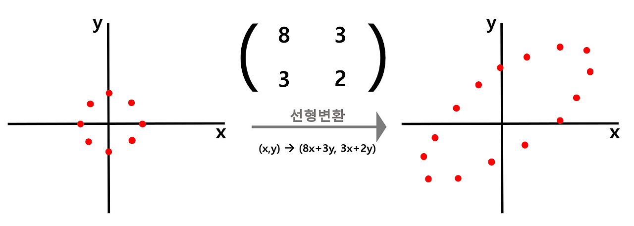
: 선형변환 관점에서 바라본 covariance matrix
🡆 원점을 기준으로 골고루 퍼져있는 normal distributied 데이터에 covariance matrix를 곱해서 선형변환을 수행해주면, 아까 봤던 것처럼 covariance matrix의 특성에 맞게 데이터가 쭉 늘어나는 형태로 변하는데, 이를 "shearing"이라고 한다.

Eigenvector, Eigenvalue

• 고유벡터(Eigenvector)
  • 행렬 A 에 의해 Linear Transformation(선형변환) 되는 수많은 벡터들 중에, 변환되기 전과 변환된 후의 벡터 방향이 똑같은 벡터
  • N 차원 데이터에서는 N개의 Eigenvector/Eigenvalue가 나온다.

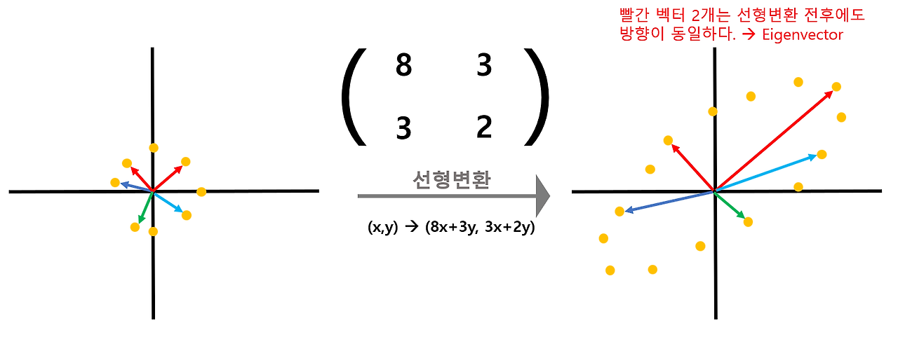
→ 단위원을 이루던 벡터는 오른쪽과 같이 1,3사분면에 걸쳐있는 넙적한 찌그러진 원이 될 것이다. 변환된 수많은 벡터들 중, 빨간색으로 표시된 벡터 2개만은 변환 전과 후의 방향이 동일한데 이 두 개의 백터가 해당 선형 시스템 방정식에 대응하는 "Eigenvector"이며, 이때 Eigenvecotr의 변환 전과 후의 길이 변화 비율을 "Eigenvalue"라고 한다.

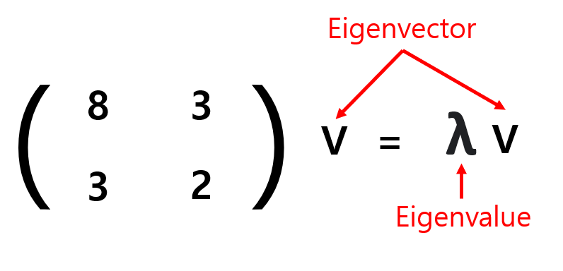
: 선형 변환이 되기 전과 후의 방향이 같은 벡터 v가 Eigenvector이며, 변화되는 길이의 비율 λ값이 Eigenvalue이다.

범주형 데이터 수치형으로 변환하기

• 머신러닝의 사이킷런 라이브러리는 문자열 값을 입력 값으로 처리하지 않기 때문에 모델을 학습시키기에 앞서 범주형 데이터를 모두 숫자형으로 변환해야 함

범주형 인코딩(Categorical Encoding)

• 텍스트로 이루어진 범주형 데이터를 수치형 데이터로 변환
• 인코딩하는 이유
  • 데이터 양이 방대한 경우 텍스트로 이루어진 범주형은 수치로 변환해줘야 데이터 처리속도가 향상됨
    • 참고
  • 컴퓨터가 가장 이해하기 쉬운 언어인 숫자로 바꿔주는 게 좋다

레이블/라벨 인코딩(Label Encoding)

• 범주형 데이터에 숫자 레이블/라벨을 할당
  = 범주마다 번호를 매김
  (예) 월요일은 1, 화요일은 2, 수요일은 3, …
• 숫자의 차이가 모델에 영향을 주지 않는 트리 계열 모델에 적용하면 좋음(의사결정나무, 랜덤포레스트)
• 숫자의 차이가 모델에 영향을 미치는 선형 계열 모델에는 적용하지 않는 것이 좋음(로지스틱 회귀, SVM, 신경망 등)

pd.factorize()

• 판다스의 factorize() 매서드
• 범주형 데이터에 숫자 라벨을 붙여 인코딩할 수 있음
  • 결과를 튜플 형태로 반환하기 때문에 형태를 바꿔 새로운 컬럼으로 추가해줘야 함
  • 데이터프레임에서 먼저 출현한 순서대로 0부터 번호 붙임 → 알파벳 순서가 아님! 주의!

df['새로운레이블인코딩컬럼명'] = pd.factorize(df['인코딩할기존컬럼명'])[0].reshape(-1,1)

LabelEncoder()

• 사이킷런(scikitlearn)의 LabelEncoder 모듈을 이용하면, 알파벳 순서대로 알아서 라벨링함

  • 문자열(범주형) 값을 내림차순 정렬 후 0부터 1씩 증가하는 값으로 변환

• 활용 방법

  • fit() : 어떻게 변환할 것인지에 대해 학습
  • transform() : 문자열을 숫자로 변환
  • fit_transform() : 학습과 변환을 한 번에 처리
  • inverse_transform() : 숫자를 다시 문자열로 변환
  • classes_ : 인코딩한 클래스 조회

# 사이킷런 패키지의 인코더 모듈 가져오기
from sklearn.preprocessing import LabelEncoder
le = LabelEncoder()

# LabelEncoder는 원래 데이터프레임에 인코딩 결과를 붙여서 반환
df['새로운레이블인코딩컬럼명'] = le.fit_transform(df['인코딩할기존컬럼명'])

원핫 인코딩(OneHot Encoding)

• 범주별로 컬럼을 만들어서 컬럼 안에 1 아니면 0 넣기
• 한 컬럼에만 1(True)이 들어가고, 나머지 컬럼은 0(False)가 들어가는 방식
• N개의 클래스를 N차원의 One-Hot 벡터로 표현되도록 변환
  • 고유값들을 피처로 만들고 정답에 해당하는 열을 1로 나머지는 0으로 표시
• 숫자의 차이가 모델에 영향을 미치는 선형 계열 모델에 주로 사용

pd.get_dummies()

• 판다스의 get_dummies() 메서드를 사용하면 빠르게 원핫 인코딩 가능
• 기본 결과값은 True/False로 채워서 나오기 때문에 1/0으로 채우고 싶다면 dtype=int 넣기

pandas.get_dummies(DataFrame \[, columns=\[변환할 컬럼명]])
→ DataFrame 에서 범주형 컬럼만 변환

OneHotEncoder()

• 사이킷런의 OneHotEncoder 모듈을 사용
• 활용 방법
  • fit() : 어떻게 변환할 것인지에 대해 학습
  • transform() : 문자열을 숫자로 변환
  • fit_transform() : 학습과 변환을 한 번에 처리
  • get_feature_names() : 원핫인코딩으로 변환된 컬럼의 이름을 반환
• DataFrame을 넣을 경우 모든 변수들을 변환하기 때문에 범주형 컬럼만 처리하도록 해야 함

예시: Label Encoding

라이브러리 및 데이터 로드

import numpy as np
import pandas as pd
from sklearn.preprocessing import LabelEncoder
from sklearn.model_selection import train_test_split
from sklearn.tree import DecisionTreeClassifier
from sklearn.metrics import accuracy_score

cols = ['age','workclass','fnlwgt','education',\
'education-num','marital-status', 'occupation',\
'relationship','race', 'gender','capital-gain',\
'capital-loss', 'hours-per-week','native-country',\
'income']
url = 'http://archive.ics.uci.edu/ml/machine-learning-databases/adult/adult.data'
df = pd.read_csv(url, header=None, names=cols, na_values=' ?')
# df.isnull().sum()
df = df.dropna() # 결측치 제거

• 데이터셋: adult.data
  • 1994년 인구조사 데이터베이스에서 추출한 미국 성인의 소득 데이터셋
• target: $50,000 이하인지 초과인지를 나타내는 income 변수

encoding_columns = ['workclass','education',\
'marital-status', 'occupation',  'relationship',\
'race','gender','native-country', 'income']
not_encoding_columns = ['age','fnlwgt', 'education-num',\
'capital-gain', 'capital-loss','hours-per-week']

• 범주형 변수와 연속형 변수를 각각 encoding_columns 와 not_encoding_columns 리스트에 할당

범주형 데이터 변환

enc_classes = {} 
def encoding_label(x):   
    # x: 범주형 타입의 컬럼(Series)
    le = LabelEncoder()
    le.fit(x)
    label = le.transform(x)
    enc_classes[x.name] = le.classes_   
    # x.name: 컬럼명
    return label

• 레이블 인코딩을 처리할 함수 생성
  • 레이블 인코딩은 1차원 배열 (리스트, ndarray, Series) 단위로 처리하기 때문에 x 값에는 범주형 타입의 컬럼을 넣어주면 됨
  • 이 과정에서 encclasses 딕셔너리에는 x.name (컬럼명) 이 key 값, le.classes 가 value 값으로 저장됨

# 함수를 데이터셋에 적용한 결과
d1 = df[encoding_columns].apply(encoding_label)

# 연속형 변수에는 함수 적용 X
d2 = df[not_encoding_columns]

data = d1.join(d2)

merge와 join의 사용법 비교

merged_example = pd.merge(df1, df2, left_index=True,\
						  right_index=True)
joined_example = df1.join(df2)

• merge를 사용할 때는 left_index와 right_index 파라미터를 True로 설정하여 인덱스를 기준으로 결합하도록 지정
• join은 기본적으로 인덱스를 기준으로 작동하기 때문에 별도의 지정 없이 바로 사용
  🡆 join과 merge 모두 강력한 데이터프레임 결합 도구로 사용하는 상황과 요구 사항에 따라 적절한 방법을 선택해야 함!

데이터셋 분할

X = data.drop(columns='income')
y = data['income']
X_train, X_test, y_train, y_test = train_test_split(X, y, test_size=0.3, \
                                                    stratify=y, random_state=1)

• 범주형 데이터를 처리한 이후 데이터셋을 분할하여 모델을 적용하고 정확도를 평가

모델 생성 및 학습, 평가

tree = DecisionTreeClassifier(max_depth=9)
tree.fit(X_train, y_train)
pred_train = tree.predict(X_train)
pred_test = tree.predict(X_test)
acc_train = accuracy_score(y_train, pred_train)
acc_test = accuracy_score(y_test, pred_test)
print(f'학습: {acc_train}, 테스트: {acc_test}')
# 출력 결과
# 학습: 0.8621702268744376, 테스트: 0.8507017349983423

예시: One-Hot Encoding

범주형 데이터 변환

from sklearn.preprocessing import OneHotEncoder
from sklearn.linear_model import LogisticRegression

df_cols = ['age','workclass','education', 'occupation', 'gender', \
           'hours-per-week', 'income']
adult_df = df[df_cols]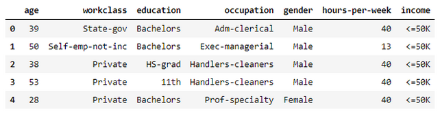

• df_cols에 해당하는 컬럼들만 불러와 원핫 인코딩 적용
• target 데이터인 income 변수는 레이블 인코딩으로 처리

# income 을 제외한 나머지 컬럼 - One-Hot Encoding
X = pd.get_dummies(adult_df[adult_df.columns[:-1]])

# income 컬럼 - Label Encoding
le = LabelEncoder()
y = le.fit_transform(adult_df['income'])
le.classes_
# 출력 결과
# array([' <=50K', ' >50K'], dtype=object)

OneHotEncoder 사용

##### 참고1 #####
ohe = OneHotEncoder()
ohe.fit(adult_df[..., np.newaxis])
ohv = ohe.transform(adult_df[..., np.newaxis])
ohv.toarray()

##### 참고2 #####
ohe = OneHotEncoder(sparse=False)
ohe.fit(adult_df[..., np.newaxis])
ohv = ohe.transform(adult_df[..., np.newaxis])
pd.DataFrame(ohv, columns=ohe.get_feature_names())

• OneHotEncoder 모델을 생성할 때 sparse 를 False 로 주지 않으면 scipy 의 csr_matrix (희소행렬 객체) 로 반환되므로, 참고1의 경우와 같이 toarray() 함수를 이용해 ndarray 로 변환해야 합니다.
• 희소행렬은 대부분 0으로 구성된 행렬과 계산이나 메모리 효율을 이용해 0이 아닌 값의 index만 관리하는 특징이 있습니다.

데이터셋 분할

X_train, X_test, y_train, y_test = train_test_split(X, y, stratify=y, \
                                                    random_state=1)

모델 생성 및 학습, 평가

lr = LogisticRegression(max_iter=1500)
lr.fit(X_train, y_train)
pred_train = lr.predict(X_train)
pred_test = lr.predict(X_test)
print(accuracy_score(y_train, pred_train))
print(accuracy_score(y_test, pred_test))
# 출력 결과
# 0.8086733566155342
# 0.8042699907174115