flatten과 revel의 차이 | 메모리 관리(.copy() vs. .view())

• 차이를 이해하기 위해서 메모리 공유에 대한 개념부터 알아야 함

.copy()

import numpy as np

a=np.arange(5) # array([0,1,2,3,4])
b=a.copy()

b[0]=100

• 5개의 원소를 가진 배열을 a 변수에 넣고, 이 값을 복사(copy)해 다시 b에 넣은 후 b[0]의 값을 바꾼 경우 a, b의 값은 어떻게 나올까?
  • print(a) → [0,1,2,3,4]
  • print(b) → [100,1,2,3,4]
• copy 함수로 복사한 경우 서로 다른 메모리 저장소를 이용하므로 b의 값만 바뀌고 a에는 영향을 주지 않는다.

.view()

import numpy as np

a=np.arange(5) # array([0,1,2,3,4])
b=a.view()

b[0]=100

• view는 기존 값이 저장되어 있는 메모리를 같이 사용해 다른 변수에 값을 할당했다 할지라도 변경 시 다 같이 변경됨
  • print(a) → [1000,1,2,3,4]
  • print(b) → [100,1,2,3,4]

• 파이썬에서는 메모리 낭비를 줄이기 위해 view() 함수를 넣지 않고 b=a와 같이 썼을 떄 디폴트로 view() 함수처럼 메모리를 공유하도록 설정되어 있다.
  • 파이토치의 torch.tensor.view()도 동일한 개념에서 출발했기 때문에 기존의 데이터와 같은 메모리 공간을 공유하며 stride 크기만 변경하여 보여주기만 다르게 한다.
    • 따라서 contiguous해야만 동작하며, 아닌 경우 에러가 발생

import numpy as np
import torch

t = np.zeros((4,4,3)) #0으로 채워진 4x4x3 numpy array 생성 
ft = torch.FloatTensor(t) #텐서로 변환
print(ft.shape) #torch.Size([4, 4, 3])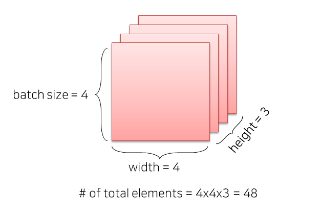

## Case 1
print(ft.view([-1, 3])) # ft라는 텐서를 (?, 3)의 크기로 변경
print(ft.view([-1, 3]).shape) 
#원소의 개수(4x4x3 = 48 개는) 유치한 채 3차원으로 맞추다보니까 결과적으론 16x3 이 됨. 

## Case 2
print(ft.view([-1, 2, 3])) # ft라는 텐서를 (?, 2, 3)의 크기로 변경
print(ft.view([-1, 2, 3]).shape) 

flatten

• 영어 뜻 그대로 '평평하게 해 주는 기능'

import numpy as np

a=np.random.randint(0,10,(2,3))

print("변경 전 a:\n", a)
b[0] = -10

print("변경 후 a:\n", a)
print("b:\n", b)

변경 전 a:
[[7 2 2]
[0 5 8]]
변경 후 a:
[[7 2 2]
[0 5 8]]
b:
[-10 2 2 0 5 8]

• flatten 변경한 b의 첫 번째 원소만 변경된 것을 확인할 수 있음
• 즉, flatten 함수는 메모리를 복사(.copy())해서 다른 공간에 저장하기 때문에 원본에는 변화가 없음
  • 이 이유 때문에 CNN 층 쌓을 때 flatten을 안 쓰고 view를 쓰는 것

In a CNN, the .view() function is preferred over .flatten() for reshaping tensors, especially when moving from convolutional layers to fully connected layers, because .view() offers more control over the reshaping process and can prevent unnecessary memory copies.

• .view() vs. .flatten()
  • .flatten()
    This function collapses all dimensions of a tensor into a single dimension, essentially creating a 1D vector. It's a simple and straightforward way to reshape a tensor, but it might not always be the most efficient way, especially when dealing with complex tensor shapes.
  • .view()
    This function allows for more fine-grained control over the reshaping process. It can reshape the tensor into any desired shape, as long as the total number of elements remains the same. Importantly, .view() can sometimes avoid creating a new memory copy of the tensor, which can be beneficial for performance, especially with large tensors. If the new shape is compatible with the original tensor's memory layout, .view() will simply provide a different view of the same data, without actually copying it.
• Why .view() is preferred in CNNs
  1. Control over Reshaping:
     When transitioning from convolutional layers (which typically output 3D or 4D tensors) to fully connected (dense) layers (which require 1D input), .view() allows you to specify the exact shape you need for the dense layer. You can reshape the tensor to be a single long vector or even a matrix if needed.
  2. Potential Memory Efficiency:
     If the new shape you're requesting with .view() is compatible with the original tensor's memory layout, it can avoid creating a new memory copy. This can lead to performance improvements, especially in larger models where memory usage is a concern.
  3. Flexibility:
     .view() can handle more complex reshaping scenarios than .flatten(). For instance, you might need to reshape a tensor into a matrix with specific dimensions rather than just a 1D vector.
• Example
  Let's say you have a 2D convolutional layer output with shape (batch_size, channels, height, width) = (32, 64, 7, 7). To feed this into a fully connected layer, you'd typically reshape it to (batch_size, features) = (32, 64 7 7).
  • Using .flatten() would simply flatten the tensor into a vector of size (32, 3136) without any regard for the original structure.
  • Using .view(batch_size, -1) (where -1 infers the correct dimension) reshapes it into (32, 3136) as well, but it might have performed a copy.
  • Using .view(batch_size, channels height width) would be clearer and potentially more efficient if the memory layout allows.
• In essence, while both functions can achieve the same reshaping, .view() provides greater control and potentially better performance, especially in the context of CNNs where memory management and flexibility are important.

np.ravel

print("변경 전 a:\n", a)
b[0] = -10

print("변경 후 a:\n", a)
print("b:\n", b)

변경 전 a:
[[7 2 2]
[0 5 8]]
변경 후 a:
[[-10 2 2]
[0 5 8]]
b:
[-10 2 2 0 5 8]

• .ravel()은 .flatten()과는 다르게 같은 메모리를 공유함
  • .ravel()을 쓰고 싶은데 메모리는 따로 쓰고 싶다면 .copy()를 사용하면 됨 → a.ravel().copy()

.base 사용

• flatten과 revel 같이 기능은 같지만 메모리상 전혀 다른 동작을 하는 api 중에는 reshape와 resize도 있음
  • 메모리상 어떤 동작을 하는지 확인할 때 필요한 것이 base
• b.base is a: b의 근간이 a에 있는지 확인
  • False → 메모리 공간을 따로 쓴다
  • True → 같은 메모리 공간을 쓴다

torch.view와 torch.reshape의 차이점
contiguous의 의미 (view, reshape, transpose, permute 이해하기)

torch.view()와 torch.reshape()

• 두 함수 모두 tensor의 형태를 바꾸는 데 사용

import torch

x = torch.arange(12)

>>> x
tensor([ 0,  1,  2,  3,  4,  5,  6,  7,  8,  9, 10, 11])

>>> x.reshape(3,4)
tensor([[ 0,  1,  2,  3],
        [ 4,  5,  6,  7],
        [ 8,  9, 10, 11]])
        
>>> x.view(2,6)
tensor([[ 0,  1,  2,  3,  4,  5],
        [ 6,  7,  8,  9, 10, 11]])

• 그러나 torch.view를 사용하다 보면 아래와 같은 에러가 발행하곤 함
  • RuntimeError: view size is not compatible with input tensor's size and stride (at least one dimension spans across two contiguous subspaces). Use .reshape(...) instead.
  • 이는 contiguous 속성 차이에 의한 것
    • view 함수는 대상 tensor가 contiguous하지 않을 경우 문제 발생

contiguous

• data들이 메모리상에서 실제로 인접해 있는지를 의미
  

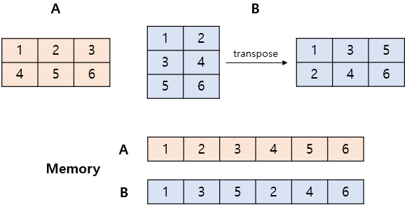
  • 메모리상에서도 순서대로 저장되어있는 상태 == contiguous 하다
  • transpose 한 뒤의 B는 그림 아래와 같이 메모리에 순서대로 저장되어 있지 않음 → 이 경우 view 사용 시 문제 발생

• contiguous 여부는 .is_contiguous() 함수로 확인 가능(True/False)

• tensor 뒤에 .contiguous()를 사용하여 강제로 contiguous하게 바꿔줄 수 있음

• 변형하려는 tensor의 상태가 확실하지 않은 경우 reshape 함수를 사용하거나, contiguous 함수를 이용해 tensor의 속성을 바꿔준 뒤 view 함수를 사용하는 것이 좋음

• 실제 우리가 다루는 array는 메모리에 저장될 때 주소 기반으로 저장됨
  

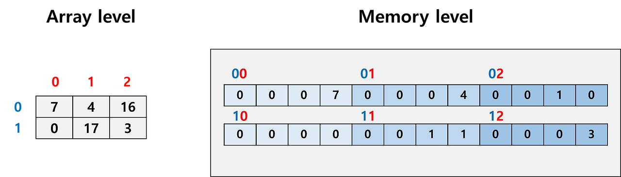
  • 우리가 코드 레벨에서 쓰는 array index는 우리가 볼 때는 단순히 0, 1, 2, 3과 같지만 메모리의 특정 주소(특정 위치)와 연결되어 있음
    • 32bit element를 담고 있는 2 x 3 array를 다룬다고 했을 때, 우리는 row index(파란색), column index(빨간색)만 보고 사용하지만 실제로는 메모리의 특정 주소를 다루는 것
    • 값은 하나지만 칸이 4개인 이유는 32bit (4byte)이기 때문에 8bit(1byte)씩 나뉘어 저장되었다는 의미 (실제로는 어떻게 쪼개냐에 따라 달라짐)
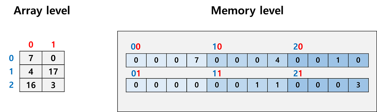
  • 만약 이 array를 transpose하고 싶다면 두 가지 방법이 존재:
    1. array index - memory address 연결은 그대로 둔 채로 저장된 값을 바꾼다
    2. 저장된 값은 그대로 두고 array index - memory를 변경한다
  • 두 번째 방법에 따라 index를 바꾸는 것이 훨씬 쉬움:
    
    • 효율성 때문에 이렇게 index-address 연결을 수정하는 식으로 데이터를 관리하는 것이 꽤 일반적인 방식

• 첫 번째 방법이든 두 번째 방법이든 우리가 코드 레벨에서 다루는 array는 전혀 변하지 않았지만(똑같은 index를 사용하면 똑같은 값을 얻을 수 있음) 분명 memory level에서는 저장된 순서의 방향이 바뀌었음 → contiguous 개념의 발생

  • memory의 row 부터 차곡차곡 채워나가는 모양에서 memory의 column부터 채워나가는 모양으로 바뀜
  • 이 뒤집힌 모양은 추후 복잡한 연산을 할 때(구체적으로는 index가 아닌 memory 주소를 직접 다룰 때) 문제를 야기할 수 있음
    • array level에서 0번 element 다음은 1번 element이지만 memory level에서 0번 element 다음은 3번 element이기 때문에 코드가 꼬일 가능성 존재

• 따라서 array level의 순서와 memory level의 순서가 나란히 정렬되어 있을 때는 contiguous, 그렇지 않을 때를 not contiguous라고 정의하고 이를 구분하기 시작함

contiguous 문제 상황

• memory address를 직접 사용하는 경우
  • python이면 이것이 흔치 않으므로 문제가 안되는데 c++ 사용 시 이는 자주 문제가 됨
  • 따라서 cython을 쓰거나 python + prebuilt c++ 를 섞어서 쓸 경우, array가 contiguous한지 확인해야 함
• pytorch를 쓸 때
  • 딥러닝 네트워크를 구현하는 과정에서 논문에 제시된 복잡한 loss function을 구현해야 하는데 이 때 수많은 tensor들을 view, reshape, transpose, permute하는 연산을 진행함
  • 해당 연산들은 어떤 tensor의 contiguous 여부를 놓친 상황에서 쓰다보면 오류가 날 수 있음 (오류가 안 나더라도 학습이 잘 안 될 수 있음)
• cuda 코드를 같이 사용할 경우
  • cuda 코드는 특히나 더 메모리 주소 관리에 민감하기 때문에 무조건적으로 contiguous tensor 상태를 유지하는 것이 좋음

view, reshape, transpose, permute

view vs reshape (안전함)

• view와 reshape 모두 torch tensor의 모양을 재배열하는 함수
• 둘의 기능은 같지만 단 하나의 차이가 존재: 입력이 not contiguous일 때 동작 여부
  • reshape는 입력이 not contiguous일 때도 동작하지만 view는 아님
  • view는 contiguous array를 재배열된 contiguous array로 만듦
    • 즉, 입력도 contiguous, 출력도 contiguous
    • 따라서 입출력 모두 contiguous가 명확한 상태일 때 사용
    • 아니라면 애초에 오류가 나기 때문에 view == contiguous 보장이라고 생각해도 됨
  • reshape는 입력은 아무거나, 출력은 contiguous
    • 여기서 중요한 것은 출력은 어쨌거나 contiguous라는 것
    • 따라서 reshape도 contiguous를 보장받을 수 있다
    • 입력이 contiguous 상태라면 입력 원본 그대로를 재배열해서 return하고, 입력이 not contiguous라면 contiguous copy를 만든 뒤, 복사본을 재배열해서 return
    • 즉, reshape() == contiguous().view()와 같다.

torch gradient 측면에서는 이러나 저러나 graph가 연결되어 있으니 걱정 안해도 된다.

transpose vs permute (위험함)

• transpose와 permute 모두 torch tensor의 dimension을 뒤바꾸는 함수
• 둘의 기능은 같고 transpose는 2개의 dimension만, permute는 여러개의 dimension을 동시에 다룰 수 있다는 차이가 있음
  • 기본적으로 transpose와 permute는 둘 다 not contiguous array를 return
    • 즉, array index - memory address 연결을 뒤 바꾸어 dimension을 재정렬하는 함수이므로 사용에 꼭 유의해야 함
• 입출력 tensor의 contiguous 여부를 잘 트래킹하면서 쓰거나, 모르겠으면 그냥 contiguous 상태로 강제 변환하고 사용하는 것을 추천