0. 기본 설정

import pandas as pd
import numpy as np
# 데이터 분포 확인을 위한 plt, sns 라이브러리 import → for 시걱화
import matplotlib.pyplot as plt
import seaborn as sns
#sklearn 에서 제공하는 데이터 셋 중 하나인 diabetes 불러오기 
from sklearn.datasets import load_diabetes
#회귀분석 라이브러리 import 
from sklearn.linear_model import LinearRegression
lr = LinearRegression()

1. 데이터 가져오기

# 데이터를 가져오고, 이름을 df 로 받아주겠습니다.
diabetes = load_diabetes()

# 자료구조 확인 - sklearn.utils._bunch.Bunch 입니다. 
# key 와 value 값으로 나뉘어 저장되어 있고, dictionary 구조와 유사합니다. 
type(diabetes), diabetes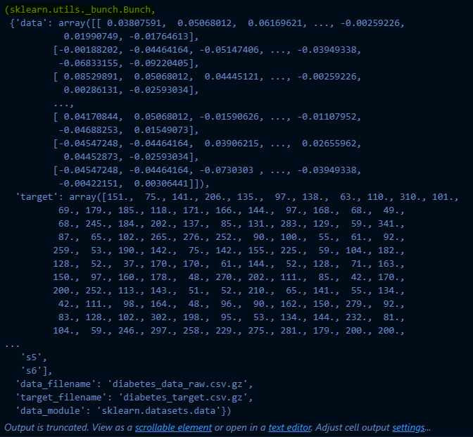

# key 를 확인해 보겠습니다. 각각의 key 값에 값이 존재합니다. 
diabetes.keys()

# 키값을 바탕으로, pandas dataframe 을 만들어 주겠습니다. 
# np.c_ 는 두 배열을 가로 방향으로 합치는 함수입니다. 
df= pd.DataFrame(data=np.c_[diabetes.data, diabetes.target], columns=diabetes.feature_names + ['target'])

# 총 442 명에 대한 나이, 성별, bmi(체질량지수).. 등을 가져왔습니다. 
df

• np.c_

• 각각을 DataFrame으로 가져온 다음 concat을 해도 됩니다!

2. 데이터 이해를 위한 탐색과 시각화(EDA)

# 히스토그램을 통한 데이터 분포 살펴보기
df.hist(bins=20, figsize=(12, 6), color='green')
plt.tight_layout()
plt.show()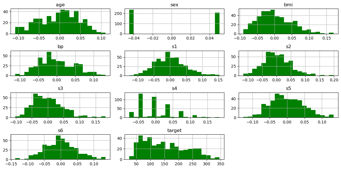

# 특성 간 상관 관계 확인하기 
# 삼각형 형식으로 보여주기
corr_matrix = df.corr()
plt.figure(figsize=(10, 8))
mask = np.triu(np.ones_like(corr_matrix, dtype=bool)) 
sns.heatmap(corr_matrix,annot=True, cmap='BrBG', linewidths=0.5, mask=mask, fmt=".2f")
plt.title("Heatmap -Using Seaborn Library")
plt.show()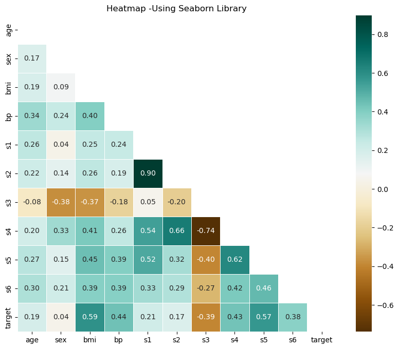

# 종속변수와 독립변수 관계 
sns.scatterplot(x='bmi', y='target', data=df, color='green', marker='*')
plt.xlabel("BMI")
plt.ylabel("Progression of Diabetes") # 당뇨병 진행 정도
plt.title("Relationship between Progression of Diabetes & BMI")
plt.show()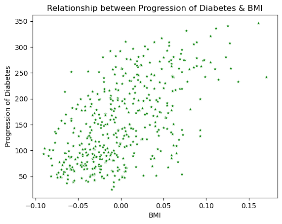

3. 모델 선택과 훈련

# Diabetes(당뇨병) 데이터셋 로드
diabetes = load_diabetes()
X = df.bmi.values
y = df.target.values

# 단순선형회귀 모델 선언
model = LinearRegression()
# 1차원 -> 2차원 변경
X = X.reshape(-1, 1)
# 모델 학습. FIT 을 사용합니다.
model.fit(X, y)


# 회귀식: y= 152.133 + 949.435*x 이 되겠습니다.
# coef 가 기울기를, intercept_가 Y 절편을 의미합니다. 
model.coef_[0], model.intercept_

.reshape(-1,1) 전 X.shape: (442,)
.reshape(-1,1) 후 x.shape: (442,1)

# 회귀선 추가하기 
plt.scatter(X, y, alpha=0.5, color='green', marker='*')
plt.plot(X, model.predict(X), color='red', linewidth=2)
plt.xlabel("BMI")
plt.ylabel("progression of diabetes") # 당뇨병 진행 정도
plt.title("The example of Linear Regression")
plt.show()

4. 모델 평가

# 회귀분석 결과 해석하기 
# 주요 해석포인트 
# 결정계수 R-squared 확인, 모형의 적합도 Prob(F-statistic) 확인, P>|t| 확인
import statsmodels.api as sm
results = sm.OLS(y, sm.add_constant(X)).fit()
results.summary()

# 메시지 Standard Errors assume that the covariance matrix of the errors is correctly specified.
# 메시지 해석 데이터 관측치의 부족으로 첨도 테스트에 문제가 있다는 경고(common notice 정도로 이해해주세요)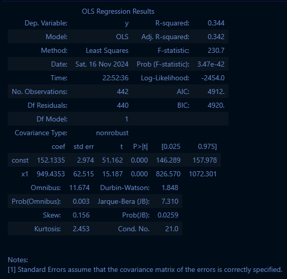

A. R제곱

• 값이 0.34정도
  • 이는 34%만큼의 설명력을 가진다고 판단할 수 있음
    • 나머지 설명되지 않는 것은 '잔차'
• 0에 가까울 수록 예측값을 믿을 수 없고 1에 가까울 수록 믿을 수 있다고 판단

B. Prob(F-statistic)

• 도출된 회귀식이 회귀분석 모델 전체에 대해 통계적으로 의미가 있는지 파악
  → F-statistic의 p-value 값은 Prob(F-statistic)으로 표현
  • 3.47e-42로 0.05보다 작기에 이 회귀식은 회귀분석 모델 전체에 대해 통계적으로 의미가 있다고 볼 수 있음
    C. P>|t|
• 각 변수가 종속변수에 미치는 영향이 유의한지 파악
• x1과 const에 대한 p-value가 0.000으로 표기 되어 있기에 0.05보다 작으므로 target을 설명하는데 유의하다고 볼 수 있음