[P&R] 03. Two Random Variables(1)

■ Joint Density & Distribution

- Joint statistics simply means the statistics of two or more random variables.

- In the discussion of joint statistics, we are interested in the intersection of events.

---

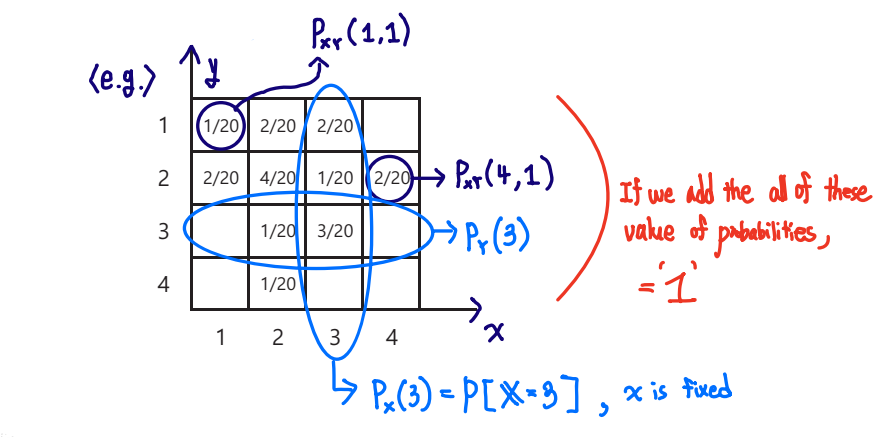
■ Joint PMF (In 1 random variable, $P_X(x) = P[X = x]$)

• $P_{XY}(x , y) = P[ X=x, Y = y]$
  

• $\sum_x \sum_y P_{XY}(x,y) = 1$

• $P_X(x) = \sum_y P_{XY}(x, y)$

• $P_Y(y) = \sum_x P_{XY}(x, y)$

• $P_{X|Y}(x|y) = P[X=x | Y=y] = \frac{P(X=x, Y=y)}{P(Y=y)} = \frac{P_{XY}(x,y)}{P_Y(y)}$

• $\sum_x P_{X|Y}(x,y) = \sum_x\frac{P_{XY(x,y)}}{P_Y(y)} = \frac{1}{P_Y(y)} \times \sum_x P_{XY}(x,y) = 1$ $(∵\sum_x P_{XY}(x,y) = P_Y(y))$

---

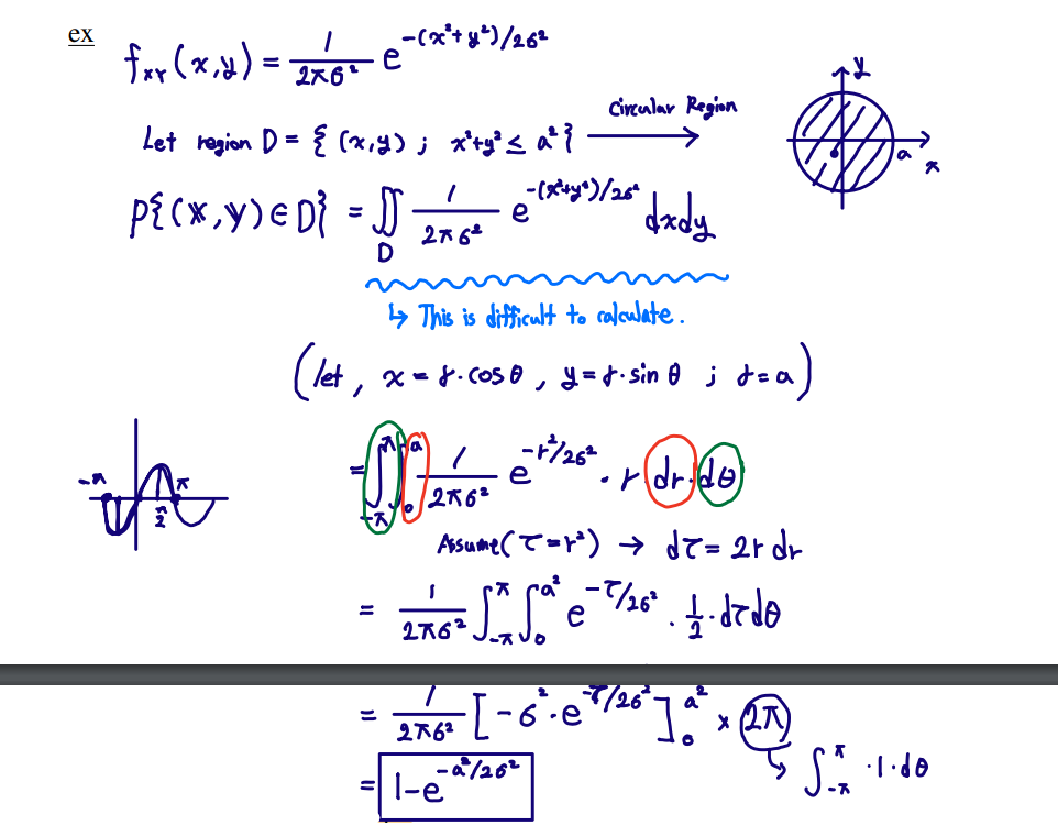
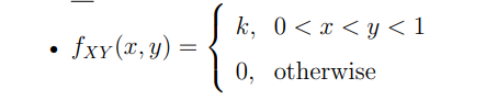
■ Joint PDF ~ $f_{XY}(x,y)$

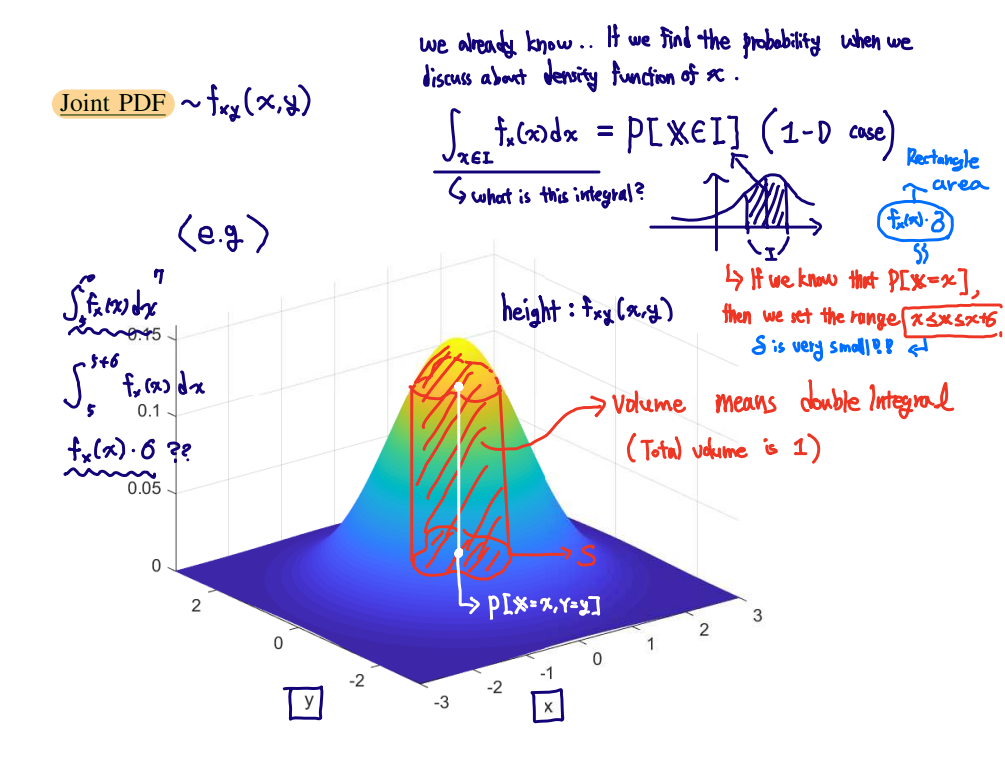
• $P[(X, Y) \in S] = \int\int_{(x,y)\in I} f_{XY}(x, y)$ $dxdy$
• $\int_{-\infin}^\infin \int_{-\infin}^\infin f_{XY}(x,y)$ $dxdy$
• $P[x \le X \le x + \delta, y \le Y \le y + \delta] \approx P[X=x, Y=y] \approx f_{XY}(x, y)\times \delta^2$
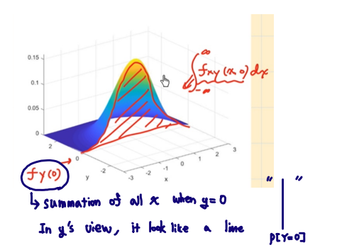
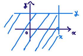
• $f_X(x) = \int_{-\infin}^\infin f_{XY}(x,y)$ $dy$
• $f_Y(y) = \int_{-\infin}^\infin f_{XY}(x,y)$ $dx$
• 

---

■ Joint Distribution

• Joint distribution of random variables $X$ and $Y$ is defined as $f_{XY}(x,y) = \frac{\delta^2}{\delta x \delta y} F_{XY}(x, y)$
  $F_{XY}(x,y) = P\{X \le x, Y\le y\}$
  

---

■ Properties

• $F_{XY}(-\infin, y) = P \{X \le -\infin, Y \le y\} = 0$
  $F_{XY}(x, -\infin) = P \{X \le -\infin, Y \le y\} = 0$
  $F_{XY}(\infin, \infin) = P \{X \le -\infin, Y \le y\} = 1$
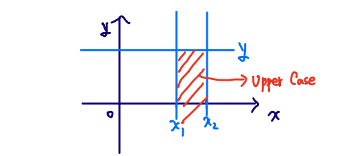
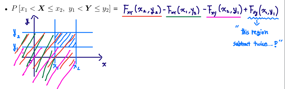
• Assume that $x_2>x_1,$ $F_{XY}(x_2,y) - F_{XY}(x_1,y) = P\{x_1\le X \le x_2 ,$ $Y \le y\}$
• Assume that $y_2>y_1,$ $F_{XY}(x,y_2) - F_{XY}(x,y_1) = P\{X \le x,$ $y_1\le Y \le y_2\}$
  
• 
• $f_{XY}(x,y) = \frac{d}{dxdy} F_{XY}(x,y)$
• $F_{XY}(x,y) = \int_{-\infin}^x \int_{-\infin}^y f_{XY}(\alpha, \beta)d\alpha d\beta$
• In comparison with joint distiribution (or joint density), the distribution of each random variable is called "marginal distribution (or density)."
• $F_X(x) = P\{X \le x\} = P\{X \le x , y \le \infin\} = F_{XY}(x, \infin)$
• $F_Y(y) = F_{XY}(\infin, y)$
• $f_X(x) = \int_{-\infin}^\infin f_{XY}(x,y)$ $dy$
• $f_Y(y) = \int_{-\infin}^\infin f_{XY}(x,y)$ $dx$
  

---

■ Independent random variables

1) Discrete random variables $X, Y, Z$ are said to be independent iff $P_{XYZ}(x, y, z) = P_X(x) \times P_Y(y) \times P_Z(z)$
Because "Joint Probability mass function" has to be equal to product of, marginal product of function.

• Also we need to satisfy other condition, $P_{XY}(x,y) = P_X(x)\times P_Y(y) \dots$
  However, we just get a 1 condition($P_{XYZ}(x, y, z) = P_X(x) \times P_Y(y) \times P_Z(z)$) -> satisfy the others condition.

  Let's suppose $\sum_Z P_{XYZ}(x, y, z) \\ \Leftrightarrow \sum_Z P_X(x) \times P_Y(y) \times P_Z(z) \\ \Leftrightarrow P_{XY}(x, y) = P_X(x) \times P_Y(y) \times \sum_Z P_Z(z)$ $(\sum_Z P_Z(z) =1)$
  Therefore, It can prove others just as 1 conditions.

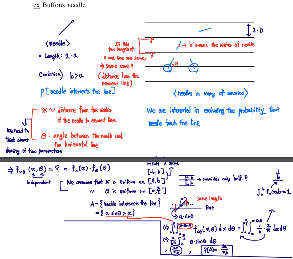
2) Continouous random variables $X, Y, Z$ are said to be independent iff
$\Leftrightarrow f_{XYZ}(x,y,z) = f_X(x) \times f_Y(y) \times f_Z(z)$
$\Leftrightarrow F_{XYZ}(x, y, z) = F_X(x) \times F_Y(y) \times F_Z(z)$
$\Leftrightarrow$ Events $\{u | X(u) \le x\}, \{u | Y(u) \le y\}, \{u | Z(u) \le z\} are independent$

Independence of RV X, Y, and Z is exactly same as independence of events $\{X \le x\}, \{Y \le y\}, \{Z \le z\}.$
Each of these events is acutally collection of sample points which is satisfied above condition.

✏️ Buffons needle example

---

■ Conditioning

Recall that

• $P_{X|Y}(x|y) = \frac{P_{XY}(x,y)}{PY(y)}$
• $P(x \le X \le x + \delta) \approx f_X(x) \times \delta$

Similarly, let's consider the following probability:

• $P(x \le X \le x+\delta | y \le Y \le y+\delta) \\ \approx \frac{P[x \le X \le x+\delta, y \le Y \le y+\delta]}{P[y \le Y \le y+\delta]} \approx \frac{f_{XY}(x,y) \times \delta^2}{f_Y(y) \times \delta}$$=\frac{f_{XY}(x,y)}{f_Y(y)} \times \delta$

• $f_{X|Y}(x|y) = f_{X|Y}(x|Y = y) = \frac{f_{XY}(x, y)}{f_Y(y)}$
  (The difference that above equation is $\delta$.)

• If $X$ and $Y$ are independent, $f_{X|Y}(x|y) = f_X(x)$

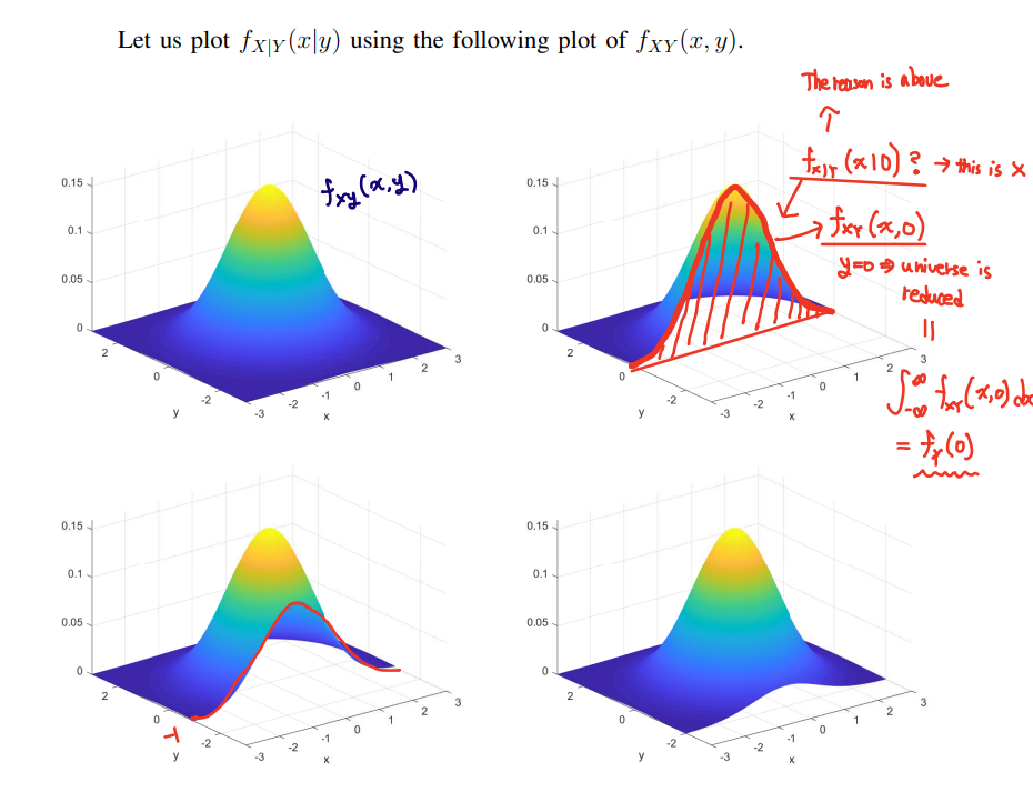
🚨Cf) $\int_{-\infin}^\infin f_{X|Y}(x|y)$ $dx = 1$ is not indicated below pic.

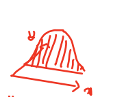
Therefore, it can not be above pic.
Because, according to the y, the result is changed not a 1.
Then, how can we find that density??
$\Rightarrow$ Make an area to 1 using normalization.
$\frac{f_{XY}(x,0)}{f_Y(0)} = f_{X|Y}(x|0)$

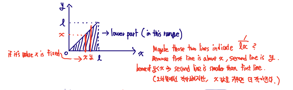
✏️ Stick-breaking example

Assumption

• Break a stick of length $l$ twice.

• Break at $X$ which is uniform in $[0,l];$ then break again at $Y$ whcih is uniform in $[0,X]$
  

• $E[Y|X = x] = x/2$ $(∵ f_{Y|X}(y|x)$'s center of gravity)

• $f_{XY}(x,y) = f_{Y|X}(y|x) \times f_X(x) = \frac{1}{lx}$ $,(0 \le y \le x \le l)$
  

• $f_Y(y) = \int_{y}^l f_{XY}(x,y)$ $dx$
  

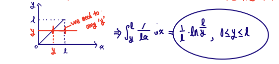
• $f_X(x) = \int_0^x f_{XY}(x, y)$ $dy$ $= \int_0^x \frac{1}{lx}$ $dy$
  $∴ 1/l, (0 \le x \le l)$

• $E[Y] = \int_0^l y \times \frac{1}{l} \times ln^{\frac{l}{y}}$ $dy$ $= \frac{l}{4}$

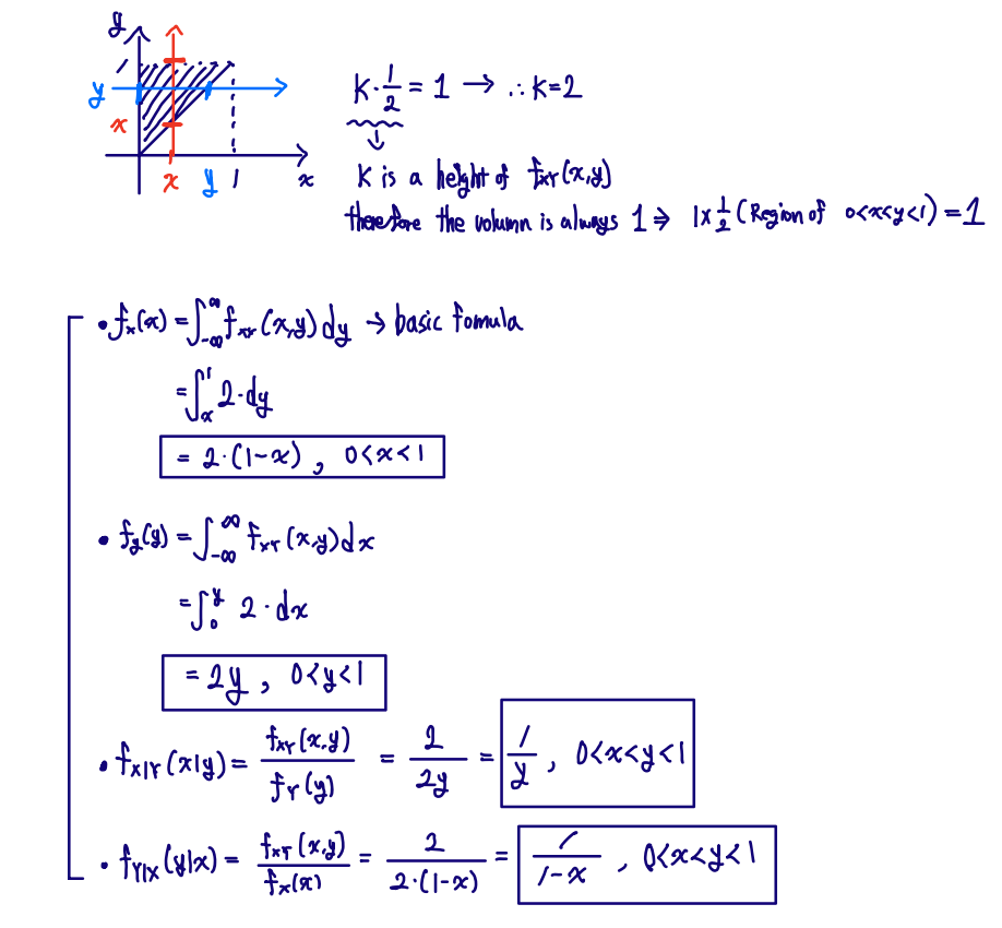
✏️ Another example

• Determine $f_{Y|X}(y|x)$ and $f_{X|Y}(x|y)$
  

---

■ Expectations

• $E[X] = \int_{-\infin}^\infin x \times f_X(x)$ $dx$
• $E[g(X)] = \int_{-\infin}^\infin g(x) \times f_X(x)$ $dx$
• $E[g(X)|A] = \int_{-\infin}^\infin g(x) \times f_{X|A}(x|A)$ $dx$
• $E[X] = \int_{-\infin}^\infin x \int_{-\infin}^\infin f_{XY}(x, y)dy$ $dx = \int_{-\infin}^\infin \int_{-\infin}^\infin x \times f_{XY}(x,y)$ $dxdy
• $E[g(X, Y)] = \int_{-\infin}^\infin \int_{-\infin}^\infin g(X, Y) \times f_{XY}(x,y)$ $dxdy$
• $E[g(X,Y) | A]= \int_{-\infin}^\infin \int_{-\infin}^\infin g(X,Y) \times f_{XY|A}(x,y|A)$ $dxdy$
• $E[X|Y = y] = \int_{-\infin}^\infin x \times f_{X|Y}(x|y)$ $dx$
• $E[X] = \int_{-\infin}^\infin E[X|Y=y] \times f_Y(y)$ $dy$

  proof)
  $E[X] = \int_{-\infin}^\infin x \times f_X(x)$ $dx$
  $\Leftrightarrow \int_{-\infin}^\infin x \int_{-\infin}^\infin f_{XY}(x,y)$ $dxdy$
  $\Leftrightarrow \int_{-\infin}^\infin \int_{-\infin}^\infin x \times f_{XY}(x, y)$ $dxdy$
  $\Leftrightarrow \int_{-\infin}^\infin \int_{-\infin}^\infin x \times f_{X|Y}(x|y) \times f_Y(y)$ $dx dy$
  $\Leftrightarrow \int_{-\infin}^\infin f_Y(y) \times E[X|Y=y]$ $dy$

We can indicates $\int_{-\infin}^\infin f_Y(y) \times E[X|Y=y]$ $dy$ to the $g(Y)$
Here, $E[X|Y=y]$ can be regarded as a random variable, being denoted by $E[X|Y]$
$∴E[X] = E[E[X|Y]]$, (Notice that inner expectation is about the X and Outer is about the Y)

✏️ Stick braking example (The range is $0 \le y \le x \le l$)

We know that $E[Y|X =x ] = \frac{x}{2}$.
And we can assume that $E[Y|X] = g(X) = x/2$.

$E[Y] = E_X[E_Y[Y|X] ],$ (we prove this above)
We can easily think $E[g(X)] = \int_{-\infin}^\infin g(x) \times f_x(x)$ $dx$.
Therefore, the expansion of above equation, $\int_{-\infin}^\infin \frac{x}{2} \times f_X(x)$ $dx$
$\Leftrightarrow \int_{0}^l \frac{x}{2} \times \frac{1}{l}$ $dx$
$∴$ $l/4$

---

본 글은 HGU 2023-2 확률변수론 이준용 교수님의 수업 필기 내용을 요약한 글입니다.