[P&R] 02. Random Variable(2)

■ Expectation

• For a discrete RV, $E[X] = \sum_{x} x \times P_X(x)$
  Indicates the center of gravity of PMF

• For a continuous RV, $E[X] = \int\limits_{-\infin}^{\infin} x \times f_X(x)$ $dx$
  

---

■ Expectation of a function of a RV

Let $Y$ = $g(X),$ then $Y$ is also a RV.
However, what is the $E[Y]?$

• For a discrete RV, $E[Y] = \sum_{y} y \times P_Y(y)$
  $\Leftrightarrow \sum_{x}g(x) \times P_X(x) \rightarrow$ We can use this when we don't know $P_Y(y)!$
  

• Similarity, for a continuous RV, $E[Y] = \int\limits_{-\infin}^\infin g(x)\times f_X(x)$ $dx$

---

■ Properties

• $E[·]$ is a linear operator. ( $∵$ Calculate the Summation or Integral)
• $E[aX] = a \times E[X]$
• $E[aX + b] = a \times E[X] + b$
• In general, $E[g(X)] \ne g(E[X])$

---

■ Variance (Distance to bias from the mean)

• $Var[X] = E[(x-\mu_x)^2] = \int\limits_{-\infin}^\infin (x-\mu_x)^2 \times f_x(x)$ $dx$
• $\sigma^2_X =-+

[x^2 -2x\mu + \mu^2] = E[x^2] - 2\mu E[X] + \mu^2 $∴ E[X^2] - \mu^2

• $\sigma_X = \sqrt{E[X^2]-\mu^2}$
• Variance measures the deviation of X from its
• $Var[·]$ is NOT a linear operator
• $Var[aX + b] = Var[Y],$ $(Y = aX +b)$
  $\Leftrightarrow E[(Y-\mu_Y)^2]$
  $\Leftrightarrow E[(aX + b - a\mu_X + b)^2,$ $($ $∵ \mu_Y = E[Y] = E[aX+b])$
  $\Leftrightarrow E[a^2(X-\mu_X)^2]$
  $\Leftrightarrow a^2\times E[(X-\mu)^2]$
  $∴ a^2Var[X]$

  Interestingly, the result shows that variance does not change by the bias 'b'
  If the RV shift by b, Mean also shift.
  Therefore the devariation(length) does not change.

---

■ Moments

• The $n^{th}$ moment of a random variable $X$ :

  $\mu_n = E[X^n]$
  $e.g)$ $m_1 = m_x$

• The $n^{th}$ central moment of a random variable $X$

  $\mu_n = E[(X-\mu_x)^n]$
  $e.g)$ $\mu_1 = 0,$ $\mu_2 = \sigma_x^2$

---

■ Conditional PMF

• $P_{X|A}(x|A) = P[X=x|A]$

• Conditional expectation $E[X|A] = \sum_{x} x\times P_{X|A}(x|A)$

---

■ Conditional PDF & Conditional CDF

• Conditional distribution $F_{X|A}(x|A) = P[X \le x|A]$
• Conditional density $f_{X|A}(x|A) = \frac{d}{dx}F_{X|A}(x|A)$
• Conditional expectation $E[X|A] = \int\limits_{-\infin}^\infin x\times f_{X|A}(x|A)$ $dx$
  

---

■ Total Expectation Theorem

Recall that $P(B) = \sum_{x=1}^n P(B|A_i)\times P(A_i)$ ~ $[A_1, \cdots, A_n]$ (Partition)

• For a discrete RV X

  $P_X(x) = P_X[X=x] = \sum_{i = 1}^n P_{X|A_i}(x|A_i)\times P(A_i)$
  $E[X] = \sum_{x} x\times P_X(x)$
  $\Leftrightarrow \sum_{i = 1}^n \sum_{x} x \times P_{X|A_i}(x|A_i)\times P(A_i)$
  $\Leftrightarrow \sum_{i = 1}^n E_{X|A_i}[x|A_i] \times P(A_i)$

• Similarity, for a continuous RV X

  $f_X(x) = \sum_{i}f_{X|A_i}(x|A_i)\times P(A_i)$ // ( If multiply the $\delta$ each of equation, the result is $P[X=x]$ )
  $E[X] = \int\limits_{-\infin}^\infin x \times f_X(x)$ $dx$
  $\Leftrightarrow \sum_{i}\int\limits_{-\infin}^\infin x \times f_{X|A_i}(x|A_i)\times P(A_i)$ $dx$
  $\Leftrightarrow \sum_{i} E_{X|A_i}[x|A_i] \times P(A_i)$ ~ Total Expectation or Expected value of $E_{X|A_i}(x|A_i)$

  Notice ... $E(X)$ is determined, but the $E(X|A_i)$ is different assumption. $\\$ Value is changed! which event assume depending on $A_i$

---

■ Memorylessness of a Geometric Random Variable

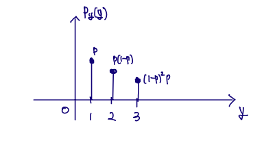
• $X$~ number of independent coin tosses until first head
• $P_X(x) = (1-p)^{x-1} \times p$ ~ Probability Mass Function of Geometric Random Variable
• $A$ (Condition) = $\{X > 2\}$
• $P_{X|A}(x|A)$
  

  • $P(A) = \sum_{x=3}^\infin (1-p)^{x-1}\times p$
    $\Leftrightarrow 1 - \sum_{x=1}^2 (1-p)^{x-1}\times p$
    $\Leftrightarrow 1-p-(1-p)\times p$
    $∴ (1-p)^2$
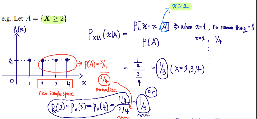
  • For a $P_{X|A}(x|A),$ we have to apply the normalization to make an area is 1.
    $P_{X|A}(x|A) = \frac{(1-p)^{x-1} \times p}{(1-p)^{2}}$
    $∴ (1-p)^{x-3}$

✏️ Example

Using the above condition, we have Head for five times $\Rightarrow$ $\{T,T,T,H,H\}$
At this time, RV X is 5.
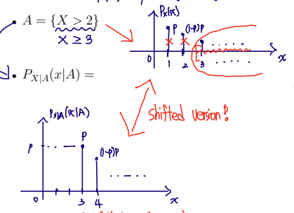
We make a condition Y is X>2 => Let $Y = X -2$ $(Y > 0),$ then $P_Y(y) = P_X(y)$
It is like the same case of $X = 3, 4, 5$ $(∵X$ is $X > 2)$ $\Rightarrow$ $Y = 1, 2, 3$

• Given that $X > 2,$ random variable $Y = X-2$ has the same geometric PMF as $X$
  In $X$ pmf, the probability same as $Y$.
  (ex) $X = Y =1,$ probability is same as $p$
• Hence, the geometric random variable is said to be memoryless, because the past has no bearing on its future behavior.
  It means even though we pick more and more the Tail, the probability of Head does not increase.

---

■ Memorylessness of exponential random variable

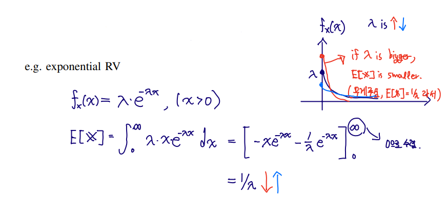
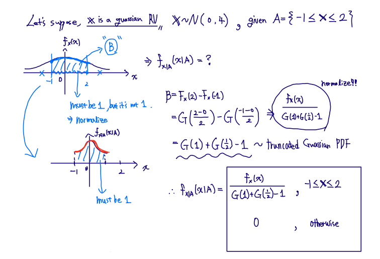
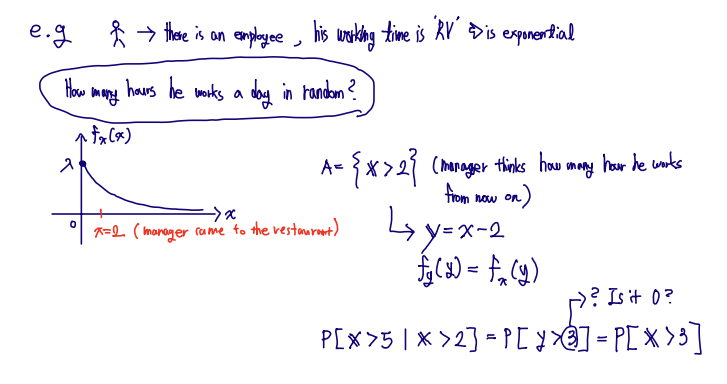
• $X$ ~ exponential random variable
• $f_X(x) = \lambda \times e^{-\lambda x},$ $(x>0)$
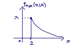
• $A = \{X > 2\}$
• $f_{X|A}(x|A) = \frac{\lambda \times e^{-\lambda x}}{e^{-2 \lambda}} = \lambda \times e^{-\lambda(x-2)},$ $(x>2)$
  
• Let $Y = X-2$ $(Y > 0),$ then $f_Y(y) = f_X(y)$ $(y>0)$
• Given that $X > 2,$ random variable $Y = X - 2$ has the same exponential PDF as $X$
• Hence, the exponential random variable is also memoryless

✏️ Example

---

■ Total Probability

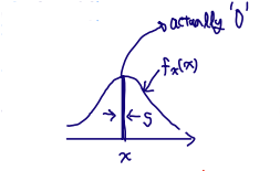
• Event A and $\{X = x\}$ $($If X is continuous, this probability is 0$)$
• Let's consider this, $P\{A, X=x\} =$ $P(A|X=x) \times P(X=x)$ $=$ $P(X=x|A)\times P(A)$
• $P(A|X=x) \times f_X(x) \times \delta$ $=$ $f_{X|A}(x|A) \times \delta \times P(A)$ $(∵$ In continuous RV, $P(X=x) = f_X(x) \times \delta)$
  $∴ P(A|X=x) \times f_X(x) = f_{X|A}(x|A) \times P(A)$
  
• Now, we can apply it like this

  $\int\limits_{-\infin}^{\infin} P(A|X=x) \times f_X(x)$ $dx$ $\cdots (1)$
  $\Leftrightarrow \int\limits_{-\infin}^{\infin} f_{X|A}(x|A) \times P(A)$ $dx$
  $\Leftrightarrow P(A) \times\int\limits_{-\infin}^{\infin} f_{X|A}(x|A)$ $dx$ $(∵P(A)$ is constant.$)$
  $∴ P(A)$
  It means that $(1)$ equation is Total Probability Theorem in continuous of $P(A)$

✏️ Example

In Coin tossing, probability that coin's face show head is P, with $f_P(p),$ $p \in [0,1]$ Find $P(head).$ (Notice that it is uniform value)

• We know that $P(head|P=x)=x$
  $(∵$ That conditional probability means we get P(head), but P(head) is P and that conditional told us P is x. $)$
• Now we define P(head) to use the total probability theorem.
  $P(head) = \int\limits_0^1 P(head|P=x) \times f_P(x)$ $dx$
• If P is uniform on [0, 1]....
  $\int\limits_0^1 x \times1$ $dx = [ \frac{1}{2} x^2]_0^1 = 1/2$
  $∴ P(head) = 1/2$

■ Bayes' theorem (continuous version)

From the equation $(1),$
$f_{X|A}(x|A) = \frac{P(A|X=x) \times f_X(x)}{P(A)}$
$∵ \frac{P(A|X=x) \times f_X(x)}{\int\limits_{-\infin}^\infin P(A|X=x) \times f_X(x)dx}$
It is used by Total Probability.

---

본 글은 HGU 2023-2 확률변수론 이준용 교수님의 수업 필기 내용을 요약한 글입니다.