동기

임베딩에 관한 생각을 하게된 이유부터 말해보겠다.
어떤 encoder 모델과 $i$번째 원본 데이터 $X^0_i$에 대해,encoder Layer $f_1$을 지나면,
$X^1 = f_1(X^0_i)$이 된다고 하자.
그러면 $X^1$은 새로운 representation으로 생각할 수 있다.

총 Layer가 L개까지 있을때,
$X^L_i = f_L(f_{L-1} \cdots \cdots f_1(X^0_i)= encoder(X^0_i)$가 된다.
그러면 $X^L$을 encoder 모델의 최종 representation이 될 것이다.

의문점

여기서 궁금증이 생겼다. $X^L_i \in \mathbb{R}^{1 \times d}$이고, 전체 trainset(= $X^0 \in \mathbb{R}^{n \times m}$)를 encoder 모델에 보내면 $X^L \in \mathbb{R}^{n \times d}$이 된다. 이때 대개 $m \gg d$이기 때문에, 정보가 lossy하게 줄어들 수 밖에 없다.
(단, len(trainset)=n)

그렇게 lossy하게 줄어든 정보인데, $X_L$의 한 차원이 constant라면 엔트로피 관점에서 $H(X) = -\sum_{x \in X} p(x) \log_2 p(x)$ 가능한 상태가 1개 이기때문에, 불확실도가 0이므로 정보 가치가 0이 된다. 만약에 이러한 차원이 여러 개라면 차원을 낭비하고 있다고 봐도 무방하다.

고민

그래서 우리가 정한 d차원을 최대한 효율적으로 활용하기 위한 방법이 무엇이 있을까생각하다가 batch normalization, covariance와 eigenvalue, PCA를 다시 고민하였다. 특히, 임베딩을 적극적으로 사용하는 contrastive learning, encoder-decoder 모델, encoder 모델에서 중요하지않을까라는 생각이 들었다.

관련 논문과 자료를 조금 읽어본뒤에 식을 정리해 보았다.

목표

Embedding을 Uniform하게 만들자!

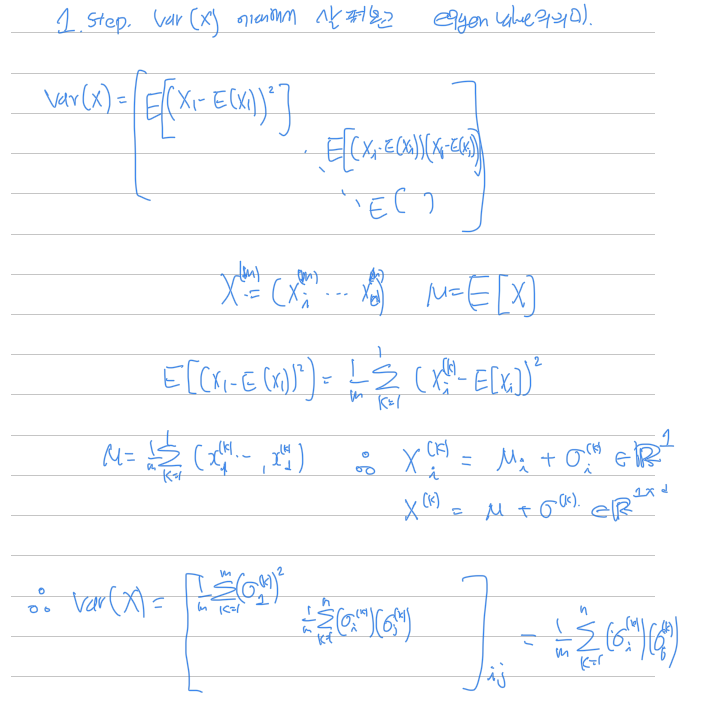
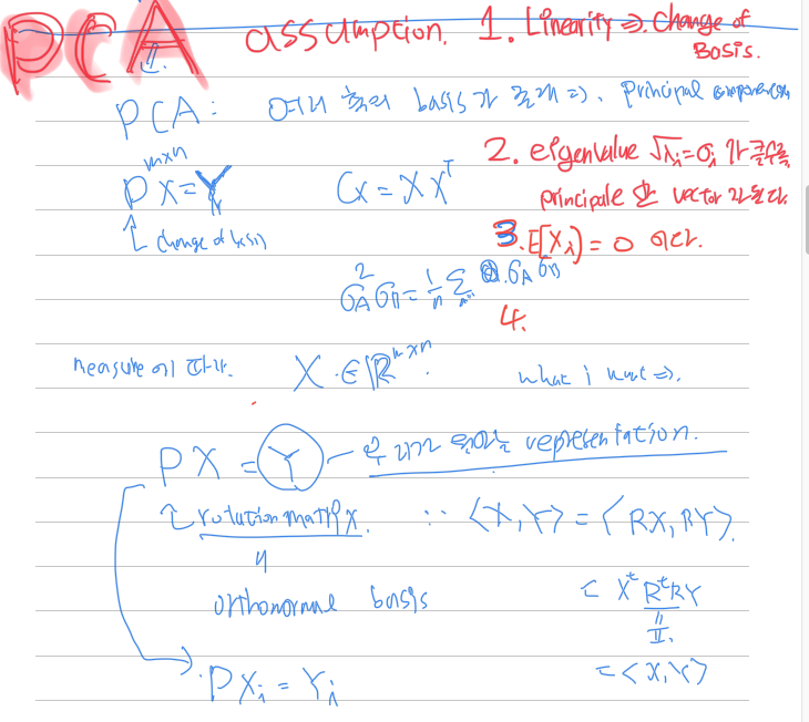
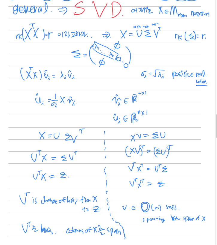
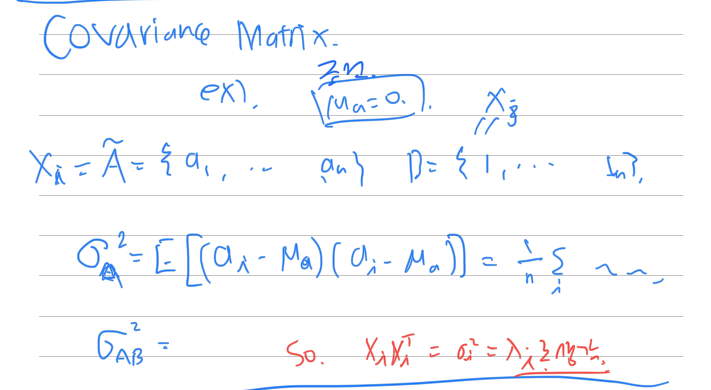
Covariance matrix

각 차원을 평균으로 빼준 경우

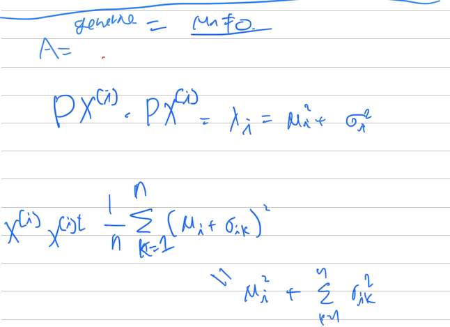
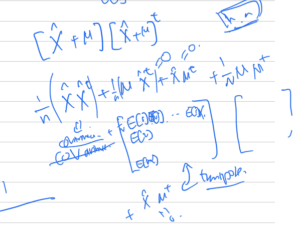
빼지 않은 경우

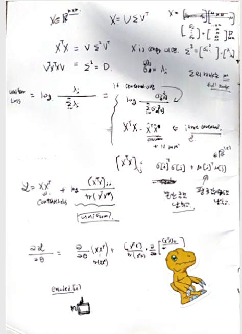
결론

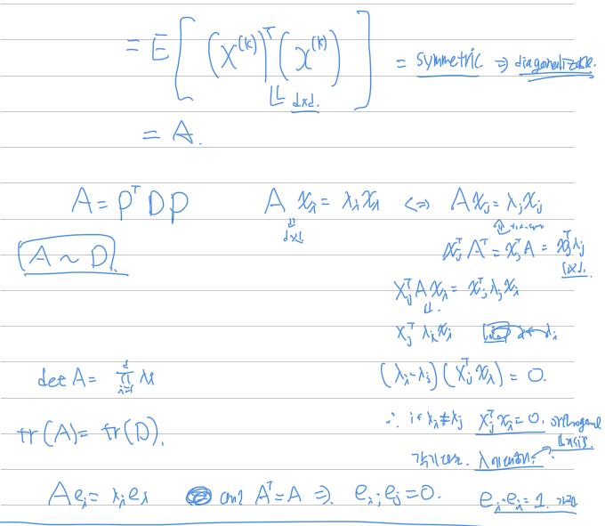
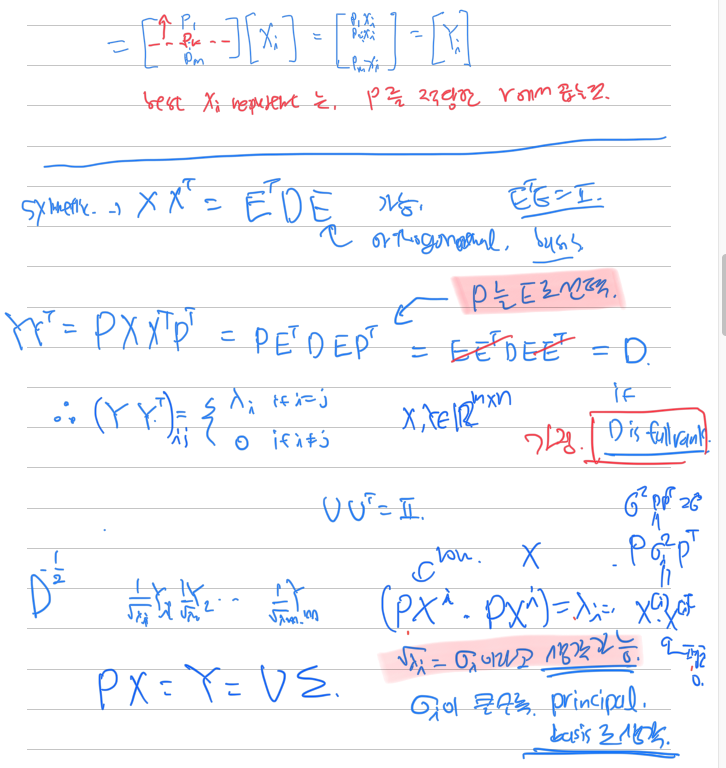
만약에 임베딩을 평균으로 빼준경우는
$X \in \mathbb{R}^{d \times n}$
$XX^T$의 eigenvalue는 $\sigma_i^2 = \lambda_i$이다. 따라서, full rank라고 할때, 최대 eigenvalue 값들을 낮추면 차원의 기저에 치우치지않을것이라고 판단하여, loss function을 다음과 같이 세웠다.

Loss function

전체 분산을 분모로, 큰 분산을 차지하는 차원의 분산을 분자로 놓아 확률을 loss function으로 사용하였다.

다만 주의할점은, embedding의 dimension보다 batch_size가 커야 한다.

그렇지 않으면 학습시에 embedding matrix의 batch_size가 최대 rank이기 때문에, 전체 임베딩 차원에 대한 분포를 알 수 없다.

위 식을 간단하게 테스트 해보기위해서 denoising autoencoder 모델에 넣어보았다.
loss에서의 $X$는 오토인코더를 통해 만들었다. 코드는 다음과 같다.

---

Code

class Autoencoder(nn.Module):
    def __init__(self):
        super(Autoencoder, self).__init__()

        self.encoder = nn.Sequential(
            nn.Linear(28*28, 128),
            nn.ReLU(),
            nn.Linear(128, 64),
            nn.ReLU(),
            nn.Linear(64, 12),
            nn.ReLU(),
            nn.Linear(12, 10),   # 입력의 특징을 3차원으로 압축합니다
        )
        self.decoder = nn.Sequential(
            nn.Linear(10, 12),
            nn.ReLU(),
            nn.Linear(12, 64),
            nn.ReLU(),
            nn.Linear(64, 128),
            nn.ReLU(),
            nn.Linear(128, 28*28),
            nn.Sigmoid(),       # 픽셀당 0과 1 사이로 값을 출력합니다
        )

    def forward(self, x):
        encoded = self.encoder(x)
        decoded = self.decoder(encoded)
        return encoded, decoded
    

import torch.nn.init as init # 초기화 관련 모듈 

def weight_initialize(m):
    if isinstance(m,nn.Linear):
        init.kaiming_uniform(m.weight.data)
        
autoencoder = Autoencoder().to(DEVICE)
autoencoder.apply(weight_initialize)
optimizer = torch.optim.Adam(autoencoder.parameters(), lr=0.005)
criterion = nn.MSELoss()
    
def train(autoencoder, train_loader):
    autoencoder.train()
    avg_loss = 0
    for step, (x, label) in enumerate(train_loader):
        noisy_x = add_noise(x)  # 입력에 노이즈 더하기
        noisy_x = noisy_x.view(-1, 28*28).to(DEVICE)
        y = x.view(-1, 28*28).to(DEVICE)

        label = label.to(DEVICE)
        encoded, decoded = autoencoder(noisy_x)
        z1,z2,z3 = torch.pca_lowrank(encoded,q=10,center=False)
        
        # A = encoded.T@encoded
        # divide = torch.trace(A)
        uniform = torch.sum(z2[:2])
        divide = torch.sum(z2)
        loss1 = uniform/divide
        
        loss2 = criterion(decoded, y)
        loss = loss1+loss2
        optimizer.zero_grad()
        loss.backward()
        optimizer.step()
        if step%20==0:
            print('uniform :',loss1,'loss2 :',loss2)
        avg_loss += loss.item()
    return avg_loss / len(train_loader)

-- 생략 ---

EPOCH = 10
for epoch in range(1, EPOCH+1):
    loss = train(autoencoder, train_loader)
    print("[Epoch {}] loss:{}".format(epoch, loss))
    
for epoch in range(1, EPOCH+1):
    loss2 = train00(autoencoder00, train_loader)
    print("[Epoch {}] loss:{}".format(epoch, loss2))

추가 Loss를 넣어준경우

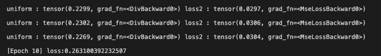
안 넣어준 경우

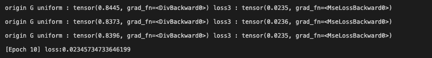
상당한 eigenvalue의 크기 차이가 있다.

다음은 두 모델의 임베딩의 eigenvector 값을 비교해 보았다.

Z = torch.tensor([])
Z0 = torch.tensor([])
autoencoder.eval()
with torch.no_grad():
    for step, (x, label) in enumerate(valid_loader):
        noisy_x = add_noise(x)  # 입력에 노이즈 더하기
        noisy_x = noisy_x.view(-1, 28*28).to(DEVICE)
        y = x.view(-1, 28*28).to(DEVICE)
        z = autoencoder.encoder(y)
        z0 = autoencoder00.encoder(y)

        Z = torch.concat((Z,z))
        Z0 = torch.concat((Z0,z0))
        if step ==15:
            break
        # label = label.to(DEVICE)
        # encoded, decoded = autoencoder(noisy_x)

print(Z.shape)
center = False
zu,zs,zu = torch.pca_lowrank(Z,q=10,center=center)
uniform = torch.sum(zs)
print(zs/uniform)

# z1,z2,z3 = torch.pca_lowrank(encoded,q=5)
print()
zu,zs,zu = torch.pca_lowrank(Z0,q=10,center=center)
uniform = torch.sum(zs)
print(zs/uniform)

위 코드는 valid set에 대해서 각 인풋을 임베딩으로 만들고, 그에 대한 eigenvalue를 구해보았다.

2차원인 경우 eigen value의 값

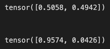
10차원인 경우

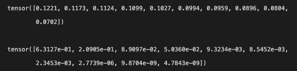
고르게 분포된 위와 달리 아래는 편향적이다.
하지만 batch normalization을 적용한 모델은 아래와 같이 편향적이지 않았다.

tensor([0.2599, 0.2530, 0.2446, 0.2426])

tensor([0.4786, 0.2771, 0.1652, 0.0790])

실험결과

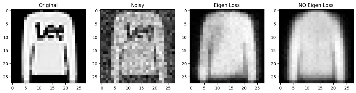
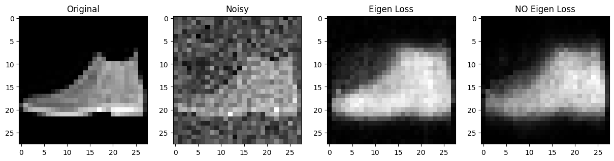
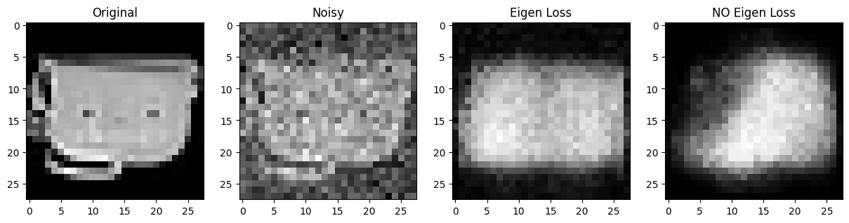
Eigen Loss vs No Eigen Loss

제가 만든 loss를 추가한 것과 아닌것을 비교해보았습니다.

Eigen Loss vs Batch Normalization

위 No Eigen Loss 모델에 layer마다 batch normalization을 적용한 경우입니다.

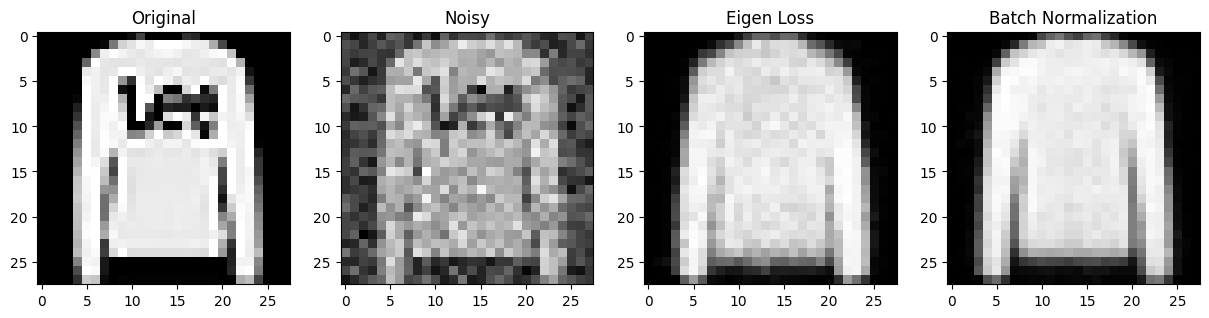
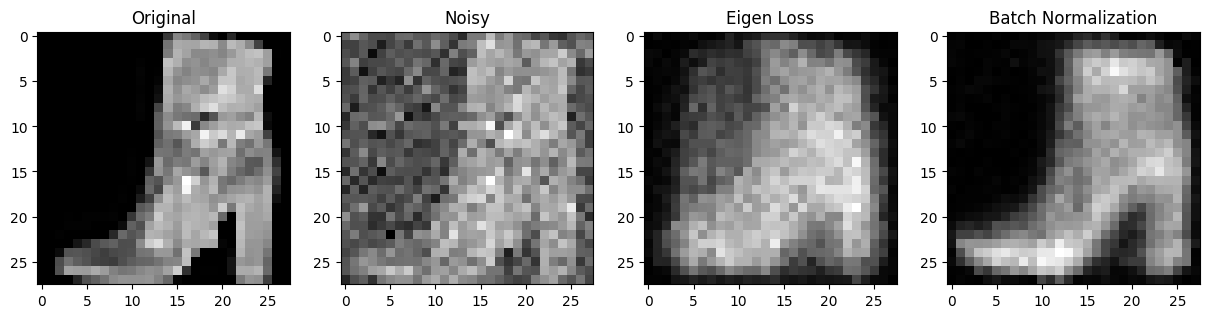
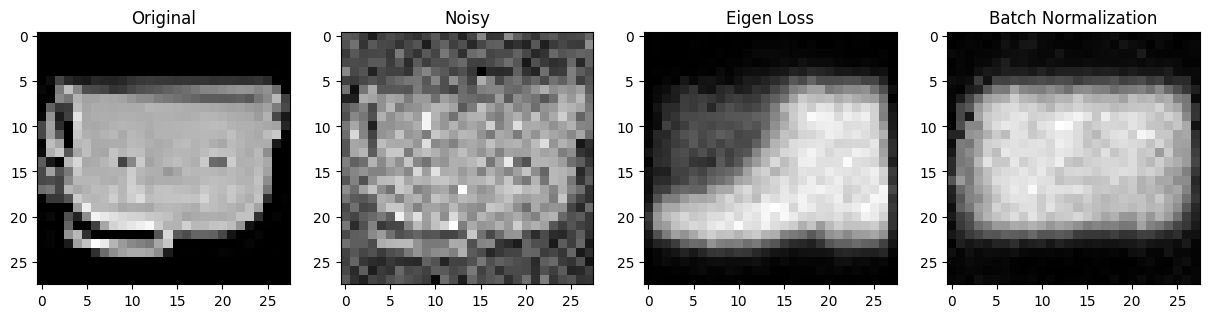
스스로 느낀 정성적인 평가를 말하면 batch normalization의 성능은 엄청나다. layer 별로 더 빠르게 학습될 뿐만 아니라, 더 정확한것 같다. 내가 만든 loss 모델과 batch normalization을 적용하지 않은 모델을 비교하면 의미가 있었고, 학습속도도 조금더 빨라진것 같았다. 하지만, batch normalization보다 효율적이냐? 라고 묻는다면 아닌것 같다... 그래서 batch normalization을 뛰어넘기 위해서는 더 연구가 필요할것 같다... 세상엔 고수들이 많다..