Deep Learning Basics
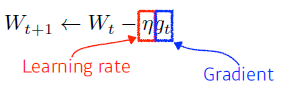
Gradient Descent
First-order iterative optimization algorithm for finding a local minimum of a differentiable function
Important Concepts in Optimization
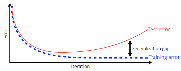
Generalization
How well the learned model will behave on unseen data
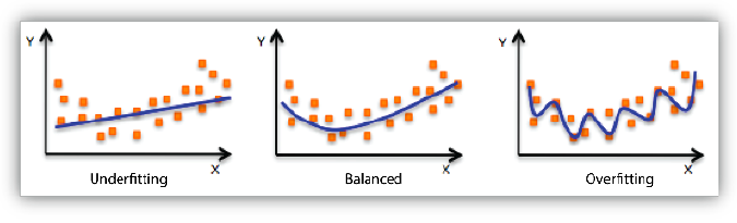
Underfitting vs. Overfitting
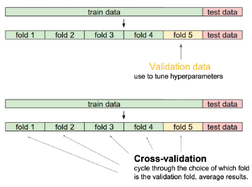
Cross-validation
Cross-validation is a model validation technique for assessing how the model will generalize to an independent (test) data set.
-
학습에 test data가 이용되서는 안 된다.
-
파라미터
최적해에서 찾고 싶은 값 (weight, bias...) -
하이퍼 파라미터
사용자가 정하는 값 (learning rate, 네트워크의 크기, loss function)
Cross-validation을 이용해 찾는다.
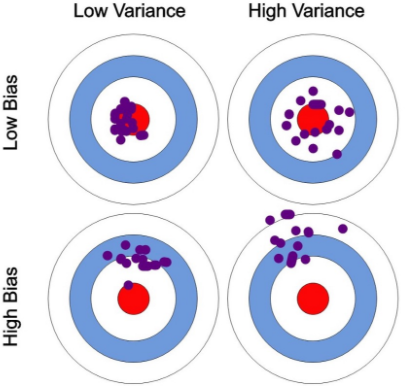
Bias and Variance
We can derive that what we are minimizing (cost) can be decomposed into three different parts: bias, variance, and noise.
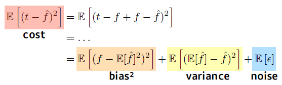
t: target (True target에 Noise가 있다고 가정)
: 신경망의 출력값
bias를 줄이려고 하면 variance가 커지고, variance를 줄이려고 하면, bias가 커지게 된다.
Bootstrapping
Bootstrapping is any test or metric that uses random sampling with replacement.
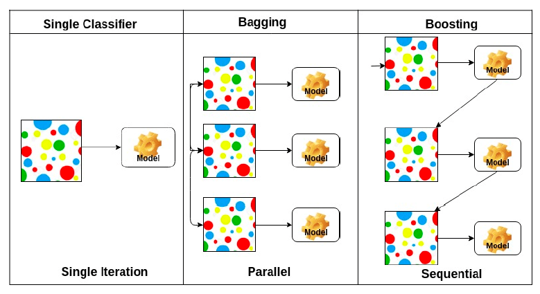
Bagging vs Boosting
-
Bagging (Bootstrapping aggregating)
- Multiple models are being trained with bootstrapping.
- ex) Base classifiers are fitted on random subset where individual predictions are aggregated (voting or averaging).
-
Boosting
- It focuses on those specific training samples that are hard to classify.
- A strong model is built by combining weak learners in sequence where each learner learns from the mistakes of the previous weak learner.
-
둘 다 여러개 모델을 쓰지만 Bagging은 여러개의 모델이 독립적으로 돌아가는데, Boosting은 weak 모델 여러개가 모여 하나의 strong 모델(결과적으로 한 개의 모델)이 된다.
Practical Gradient Descent Methods
-
Stochastic gradient descent
Update with the gradient computed from a single sample. -
Mini-batch gradient descent
Update with the gradient computed from a subset of data. -
Batch gradient descent
Update with the gradient computed from the whole data.
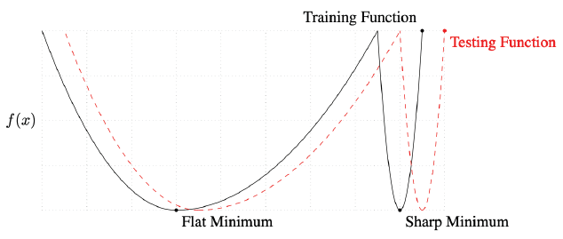
Batch-size Matters
Large batch methods tend to converge to sharp minimizers of the training and testing functions. In contrast, small-batch methods consistently converge to flat minimizers.
Gradient Descent Methods
- Stochastic gradient descent
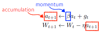
- Momentum (관성)
- Nesterov Accelerated Gradient
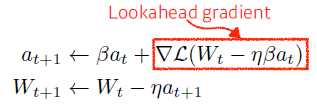
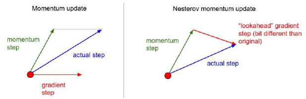
weight가 갱신된 곳에서의 gradient를 계산한다.
- Adagrad
Adagrad adapts the learning rate, performing larger updates for infrequent and smaller updates for frequent parameters.
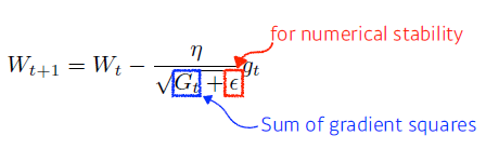
가 계속 커져 나중에는 학습이 되지 않는다.
- Adadelta
Adadelta extends Adagrad to reduce its monotonically decreasing the learning rate by restricting the accumulation window.
Exponential Moving Average
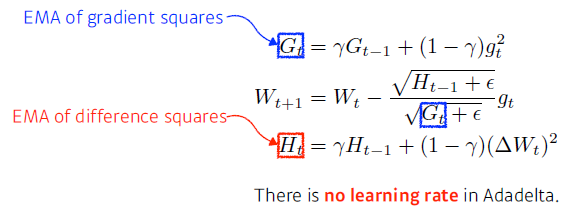
파라미터의 변화를 저장하기 때문에 GPT - 3 같이 큰 모델의 파라미터에서는 GPU 사용량이 커진다.
- RMSprop
RMSprop is an unpublished, adaptive learning rate method proposed by Geoff Hinton in his lecture.
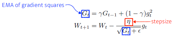
- Adam
Adaptive Moment Estimation (Adam) leverages both past gradients and squared gradients.
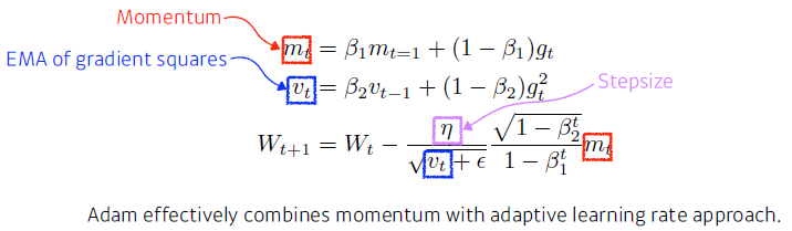
하이퍼 파라미터
: momentum을 얼마나 유지시킬지
: EMA of gradient squares
: Learning rate
: 분모를 0으로 안 만들기위한 파라미터 (default 10)
Regularization
Generalization을 위한 학습 제한
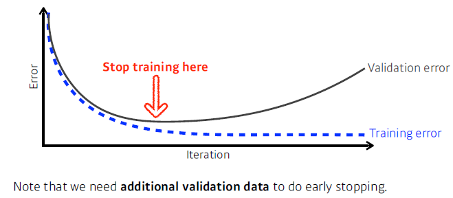
Early Stopping
Parameter Norm Penalty (Weight decay)
It adds smoothness to the function space.
- 신경망의 파라미터가 너무 커지지 않게 한다.
- 함수를 부드럽게 하면 Generalization performance가 높을 것이라는 가정
Data Augmentation
More data are always welcomed.
However, in most cases, training data are given in advance. In such cases, we need data augmentation.
Noise Robustness
Add random noises inputs or weights
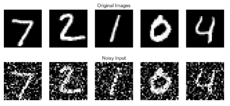
Data Augmentation와의 차이: noise를 단순히 입력에만 주는게 아니라 weight에도 적용시켜, 학습시킬 때 마다 weight에 noise가 들어간다.
Label Smoothing
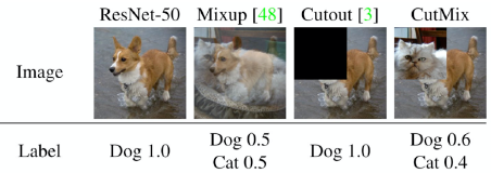
Mix-up constructs augmented training examples by mixing both input and output of two randomly selected training data.
CutMix constructs augmented training examples by mixing inputs with cut and paste and outputs with soft labels of two randomly selected training data
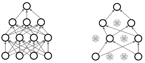
Dropout
In each forward pass, randomly set some neurons to zero.
Batch Normalization
Batch normalization compute the empirical mean and variance independently for each dimension (layers) and normalize.
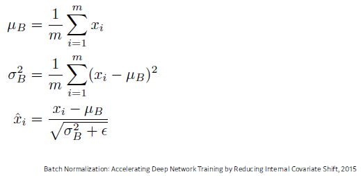
그 효과에 대해서 논란이 있지만, 일반적으로 깊은 layer의 신경망에서 성능이 많이 올라간다고 알려져있다.
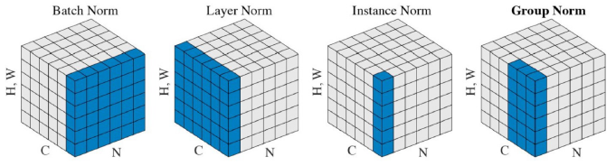
There are different variances of normalizations.
CNN
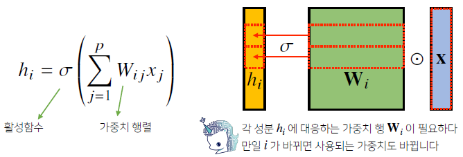
- 지금까지 배운 다층신경망(MLP)은 각 뉴런들이 선형모델과 활성함수로 모두 연결된 (fully connected) 구조였습니다.
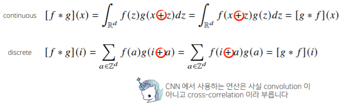
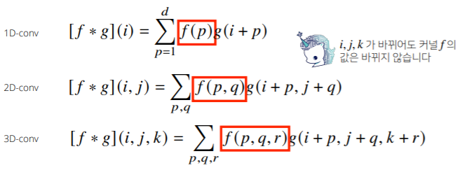
- Convolution 연산의 수학적인 의미는 신호(signal)를 커널을 이용해 국소적으로 증폭 또는 감소시켜서 정보를 추출 또는 필터링하는 것입니다.
-
커널은 정의역 내에서 움직여도 변하지 않고(translation invariant) 주어진 신호에 국소적(local)으로 적용합니다.
-
Convolution 연산은 1차원뿐만 아니라 다양한 차원에서 계산 가능합니다.
2차원 Convolution
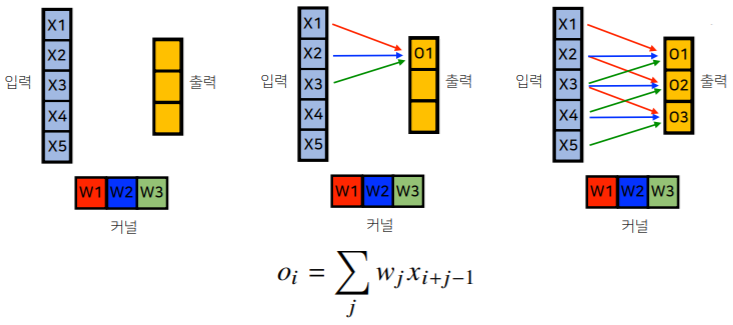
2D-Conv 연산은 커널(kernel)을 입력벡터 상에서 움직여가면서 선형모델과 합성함수가 적용되는 구조입니다.
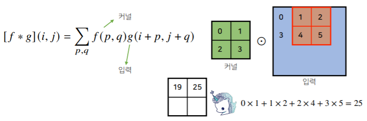
입력 크기를 ,커널 크기를 ,출력 크기를 라 하면 출력 크기는 다음과 같이 계산합니다.
(28 x 28) 입력을 (3 x 3) 커널로 2D-Conv 연산을 하면 (26 x 26)이 된다.
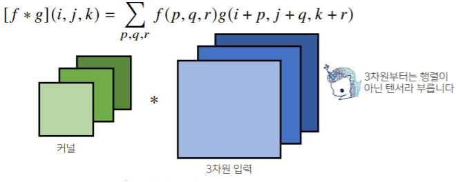
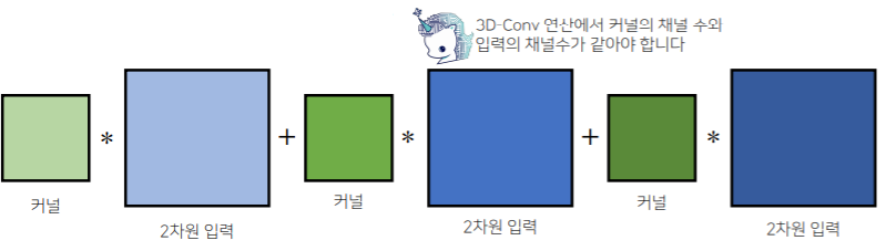
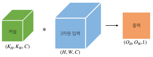
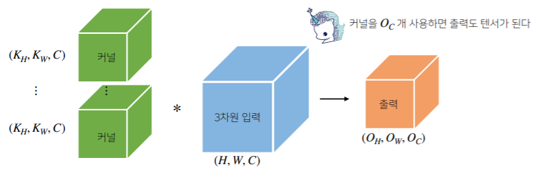
3차원 Convolution
3차원 Convolution의 경우 2차원 Convolution을 3번 적용한다고 생각하면 됩니다.
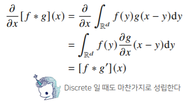
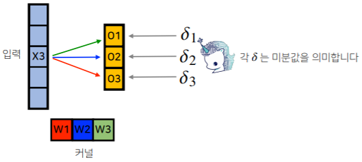
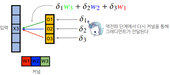
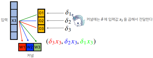
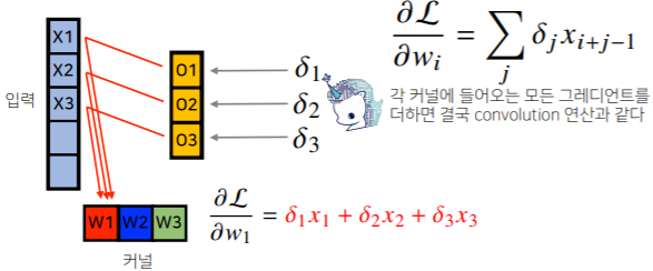
Convolution 연산의 역전파
Convolution 연산은 커널이 모든 입력 데이터에 공통으로 적용되기 때문에 역전파를 계산할 때도 convolution 연산이 나오게 됩니다.