Computer Vision
Course overview
Why is visual perception important?
- Artificial Intelligence (AI)?
The theory and development of computer systems able to perform tasks normally requiring human intelligence, such as visual perception, speech recognition, decision-making, and translation between languages.
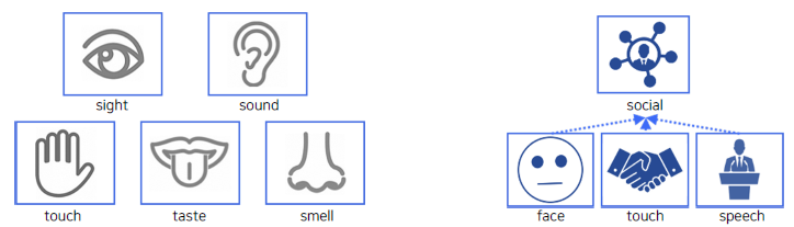
Humans learn about the world through multi-modal perception.
Perception to system?
- It’s (input, output) data
- As humans grow, we learn about the world by interacting with it.
- We gather informative signals from multi-modal association.
- Developing machine perception is still an open research area.
Why is visual perception important?
-
Sensing
About 75% of information comes through our eyes. -
Understanding
More than 50% of the brain is devoted to processing visual info.
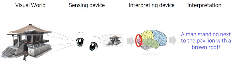
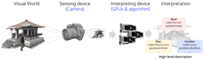
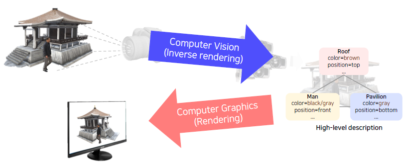
What is computer vision?
-
Visual perception & intelligence
- Input : visual data (image or video
-
Class of visual perception
-
Color perception
-
Motion perception
-
3D perception
-
Semantic-level perception
-
Social perception (emotion perception
-
Visuomotor perception, etc.
-
Also, computer vision includes understanding human visual perception capability!
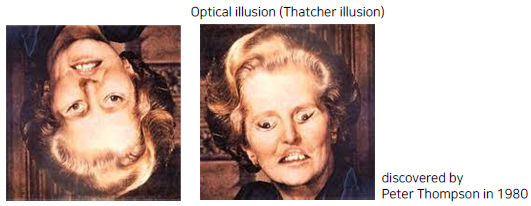
Our visual perception is imperfect.
- To develop machine visual perception,
- We need to understand the good and bad of our visual perception.
- We need to come up with how to compensate for the imperfection.
How to implement?
What you will learn in this course
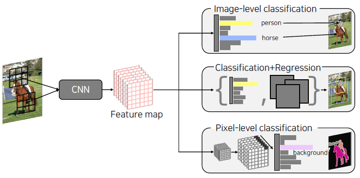
Fundamental image tasks
- Image
- Semantic segmentation
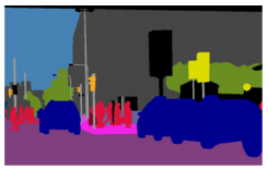
- Object detection & segmentation
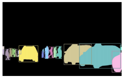
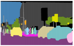
- Panoptic segmentation
Data augmentation and knowledge distillation.
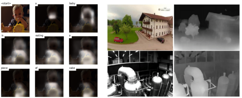
Multi-modal learning (vision + {text, sound, 3D, etc.})
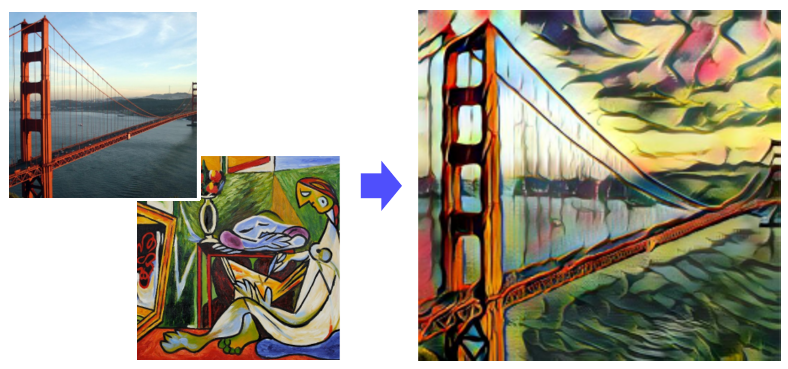
Conditional generative model
Neural network analysis by visualization
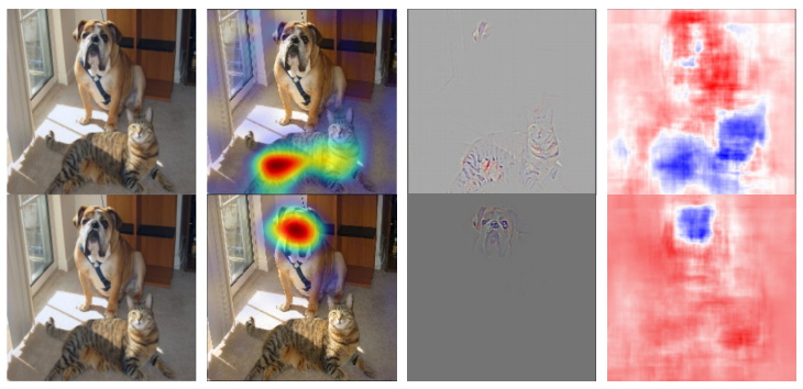
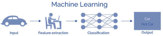
Image classification
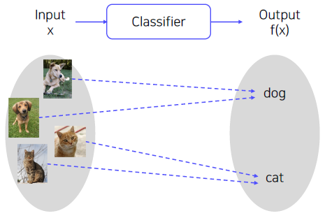
What is classification
-
Classifier
- A mapping f(.) that maps an image to a category level.
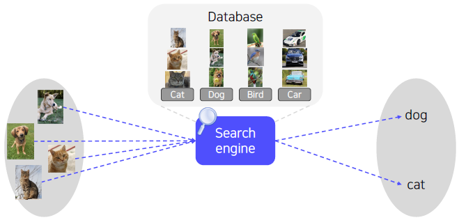
An ideal approach for image recognition
What if we could memorize all the data in the world?
All the classification problems could be solved by k Nearest Neighbors (k-NN)!
k Nearest Neighbors (k-NN)
Classifies a query data point according to reference points closest to the query.
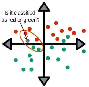
All the classification problems could be solved by k-NN!
Is it realizable?
- Time complexity (e.g., linear search)
- O(n), n = infinite
- O(n), n = infinite
- Memory complexity
- O(n), n = infinite
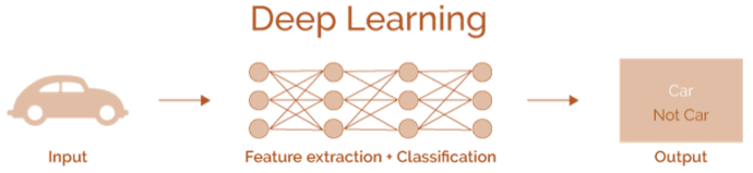
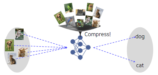
Convolutional Neural Networks (CNN)
Compress all the data we have into the neural network.
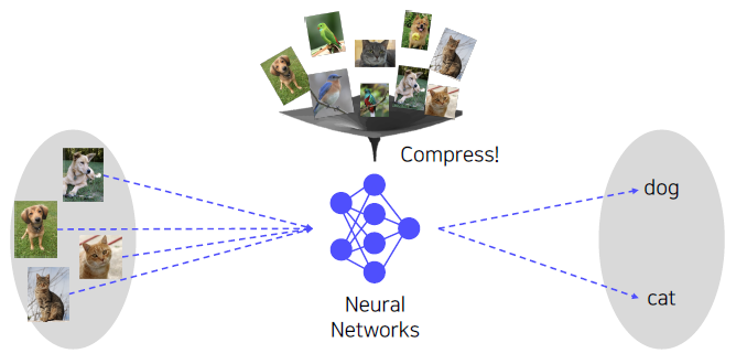
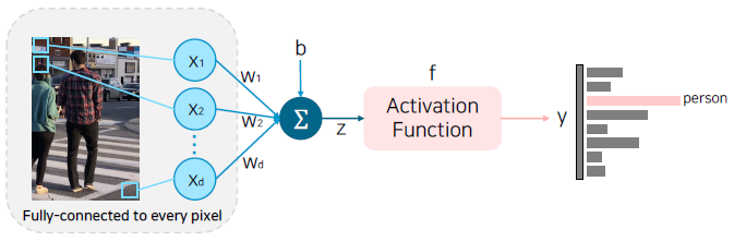
Let’s look at a simple model, perceptron, that takes every pixel of an image as input.
But, is this model suitable for solving the image classification problem?
Visualization of single fully connected layer networks.
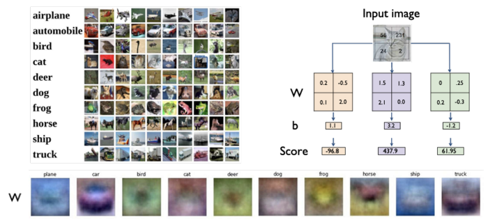
각 형상마다 W의 모습이 희미하게 관찰된다.
A problem of single fully connected layer networks.
W의 형상이 고정되기에 그 형상을 벗어나면, 다른 값으로 분류를 하게된다.
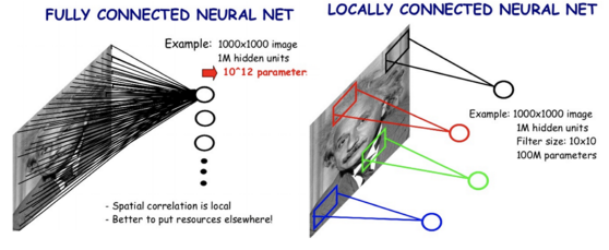
Convolution neural networks are fully locally connected neural networks.
- Local feature learning
- Parameter sharing
CNN is used as a backbone of many CV tasks.
backbone: Base network (영상의 특징을 추출)
CNN architectures for image classification
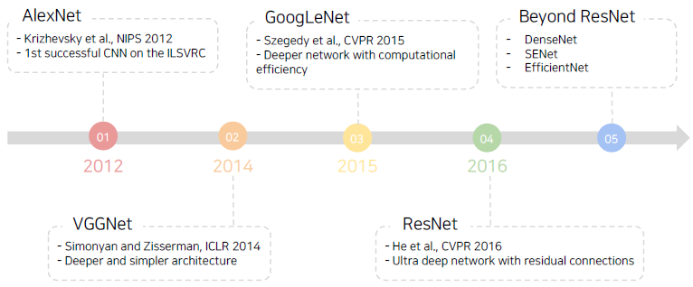
Brief History
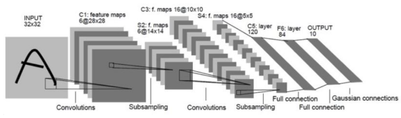
LeNet-5
A very simple CNN architecture introduced by Yann LeCun in 1998.
- Overall architecture: Conv - Pool - Conv - Pool - FC FC
- Convolution: 5x5 filters with stride 1
- Pooling: 2x2 max pooling with stride 2
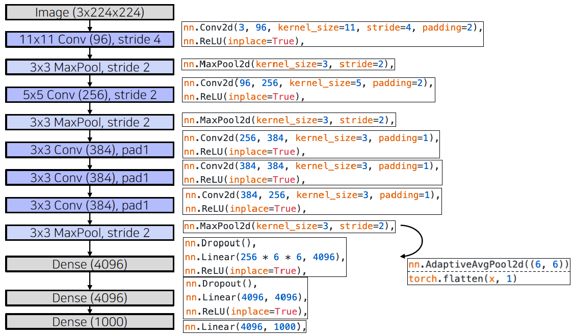
AlexNet
Similar with LeNet-5, but
- Bigger (7 hidden layers, 605k neurons, 60 million parameters)
- Trained with ImageNet (large amount of data, 1.2 millions)
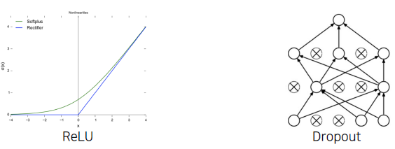
- Using better activation function (ReLU) and regularization technique (dropout)
Overall architecture
Conv - Pool - LRN - Conv - Pool - LRN - Conv - Conv - Conv - Pool - FC - FC - FC
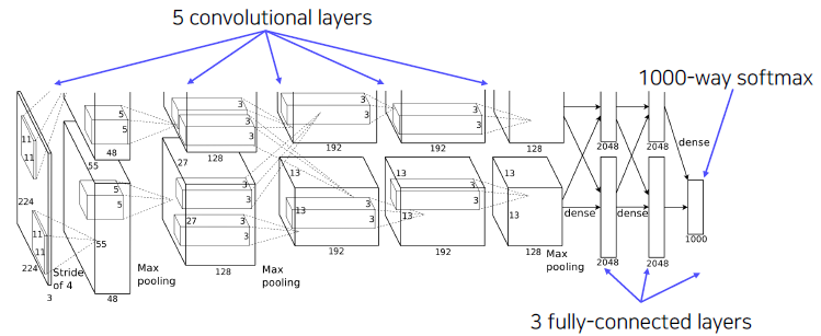
LRN(Local Response Normalizaion) is not used in this example.
Local Response Normalization (LRN)
- Lateral inhibition: the capacity of an excited neuron to subdue its neighbors.
- LRN normalizes around the local neighborhood of the excited neuron.
- Excited neuron becomes even more sensitive as compared to its neighbors.
Activation layer에서 명암을 normalization 한다.
현재는 쓰이지 않고 Batch normalization으로 대체되었다.
11x11 convolution filter
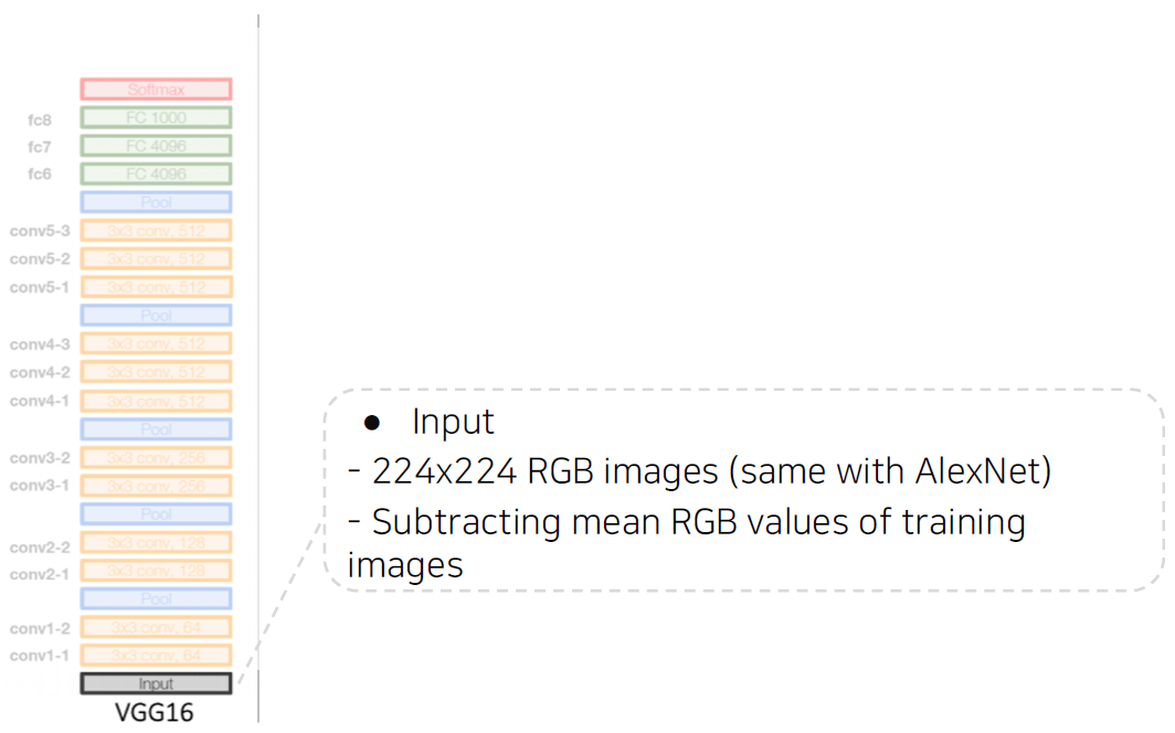
- The filter size is increased, as the input size of the image has increased.
- LeNet: 28x28
- AlexNet: 227x227
- Larger size filters are used to cover a wider range of the input image
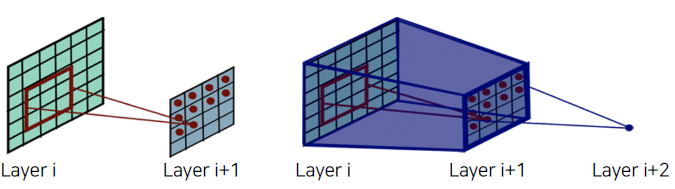
Receptive field in CNN
-
The region in the input space that a particular CNN feature is looking at
-
Suppose K×K conv. filters with stride 1, and a pooling layer of size P×P,
- then a value of each unit in the pooling layer depends on an input patch of size
- (P+K-1) (P+K-1)
VGGNet
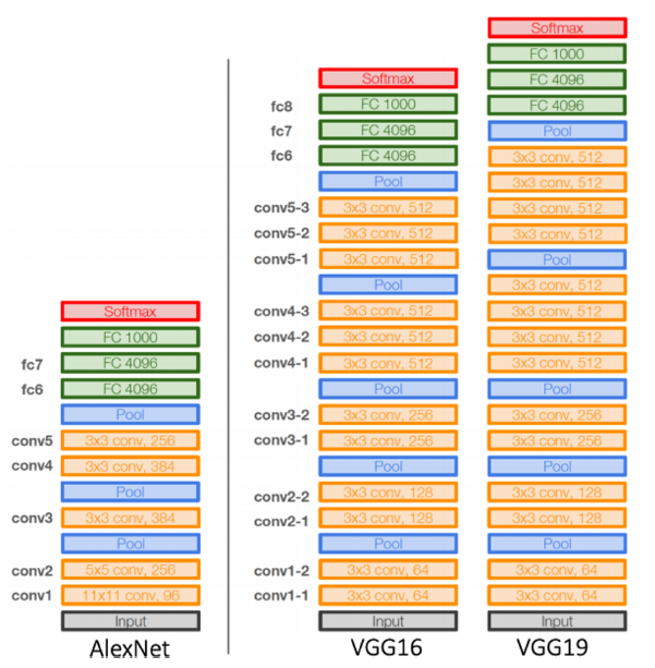
-
Deeper architecture
- 16 and 19 layers
-
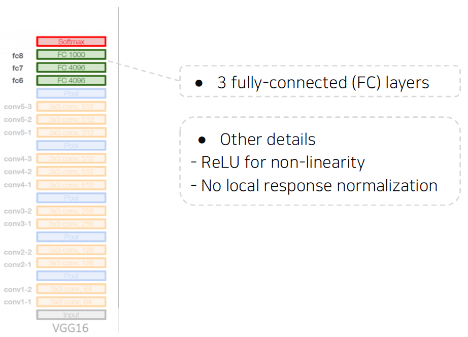
Simpler architecture
- No local response normalization
- Only 3x3 conv filters blocks, 2x2 max pooling
-
Better performance
- Significant performance improvement over AlexNet
(2nd in ILSVRC14)
- Significant performance improvement over AlexNet
-
Better generalization
- Final features generalizing well to other tasks even without fine-tuning.
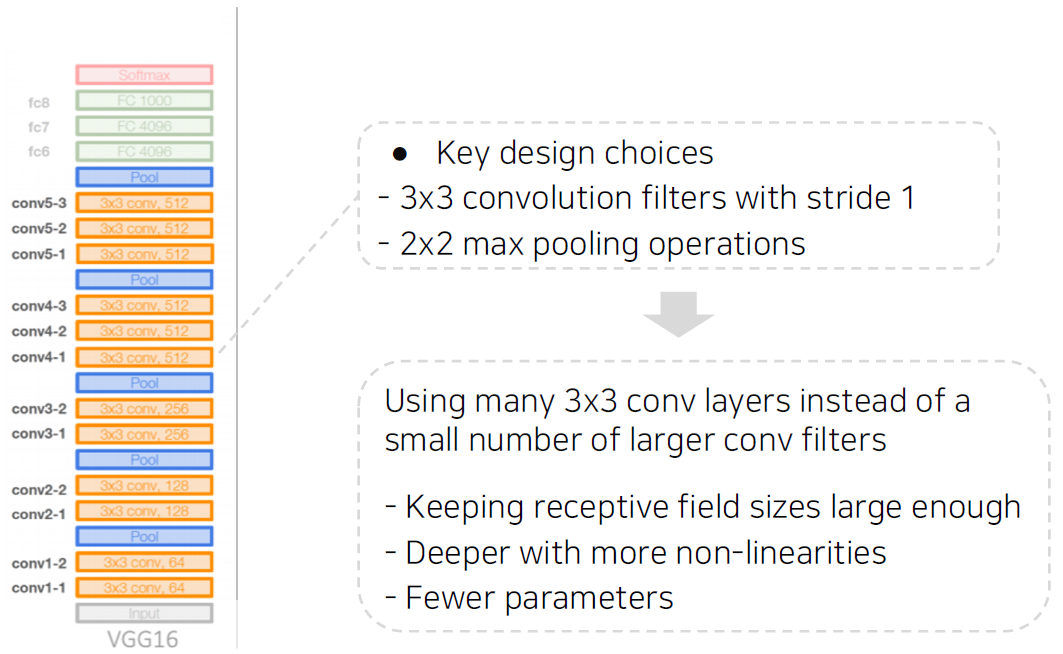
작은 conv filter를 써도 층을 깊게 쌓으면 큰 영역의 receptive field를 가진다.
Annotation data efficient learning
Data augmentation
Learning representation of dataset
- Neural networks learn compact features (information) of a dataset.
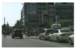
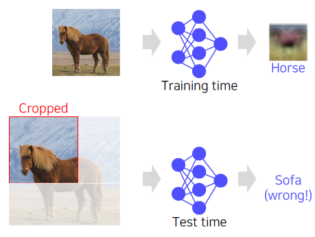
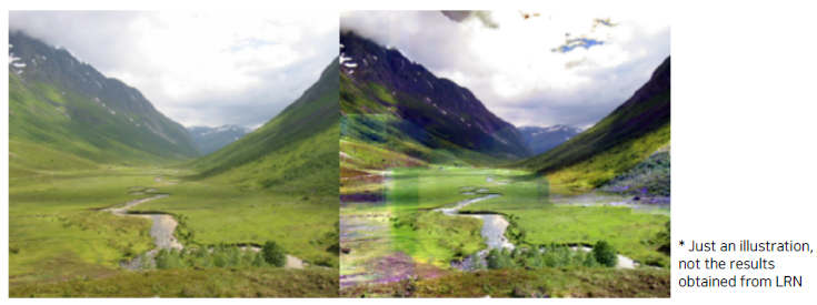
Dataset is (almost) always biased
- Images taken by camera (training data) real data
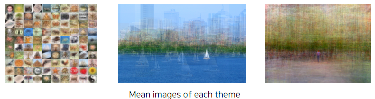
위 이미지는 각 주제별로 나오는 이미지들의 평균 데이터를 시각화한 것인데 가운데 이미지는 강이라는 이미지이고, 오른쪽 이미지는 공원이라는 이미지를 시각화한 것이다. 이를 보면 각 이미지 별로 데이터들이 편향된 것을 볼 수 있다. (사람이 보기 좋은 모양, 각도로 편향되어 있다. 사진의 용도를 생각해보면 그 이유를 알 수 있다)
The training dataset is sparse samples of real data.
- The training dataset contains only fractional part of real data.
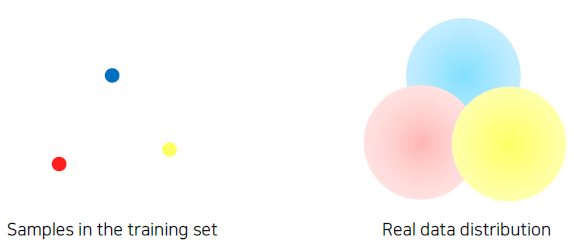
The training dataset and real data always have a gap.
- Suppose a training dataset has only bright images.
- During test time, if a dark image is fed as input, the trained model may be confused.
- Problem: Datasets do not fully represent real data distribution!
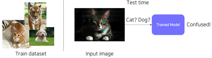
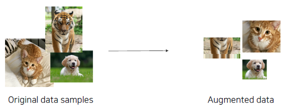
Augmenting data to fill more space and to close the gap.
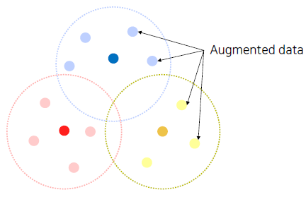
Examples of augmentations to make a dataset denser.
Data augmentation
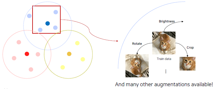
Image data augmentation
-
Applying various image transformations to the dataset
- Crop, Shear, Brightness, Perspective, Rotate …
-
OpenCV and NumPy have various methods useful for data augmentation.
-
Goal: Make training dataset’s distribution similar with real data distribution.
Various data augmentation methods
Brightness adjustment
- Various brightness in dataset.
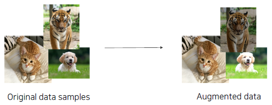
- Brightness adjustment (brightening) using NumPy.
def brightness_augmentation(img):
    # nummpy array img has RGB value(0~255) for each pixel
    img[:,:,0] = img[:,:,0] + 100 # add 100 to R value
    img[:,:,1] = img[:,:,1] + 100 # add 100 to G value
    img[:,:,2] = img[:,:,2] + 100 # add 100 to B value

    img[:,:,0][img[:,:,0]>255] = 255 # clip R values over 255
    img[:,:,1][img[:,:,1]>255] = 255 # clip G values over 255
    img[:,:,2][img[:,:,2]>255] = 255 # clip B values over 255
    return img
Rotate, flip
- Diverse angles in dataset.
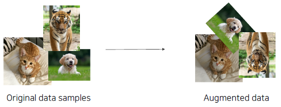
- Rotating (flipping) image using OpenCV.
img_rotated = cv2.rotate(image, cv2.ROTATE_90_CLOCKWISE)
img_flipped = cv2.rotate(image, cv2.ROTATE_180)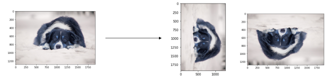
Crop
- Learning with only part of images.
- Cropping image using NumPy.
y_start = 500 # y pixel to start cropping
crop_y_size = 400 # cropped image's height
x_start = 300
crop_x_size = 800 # cropped image's width
img_cropped = image[y_start : y_start + crop_y_size, x_start + crop_x_size, :]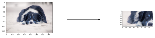
Affine transformation
변환 전후 선은 선으로 유지되며, 길이의 비율, 평행 관계 또한 유지되는 선형변환이다.
- Preserves ‘line’, ‘length ratio’, and ‘parallelism’ in image.
- For example, transforming a rectangle into a parallelogram
(See the shear transform example below)
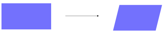
- Affine transformation (shear) using OpenCV.
rows, cols, ch = image.shape
pts1 = np.float32([[50, 50],[200,50],[50,200]])
pts2 = np.float32([[10, 100],[200,50],[100,250]])
M = cv2.getAffineTransform(pts1, pts2)
shear_img = cv2.warpAffine(image, M, (jcols,rows))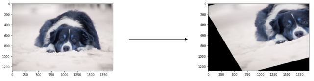
Modern augmentation techniques
CutMix
- ‘Cut’ and ‘Mix’ training example to help model better localize objects.
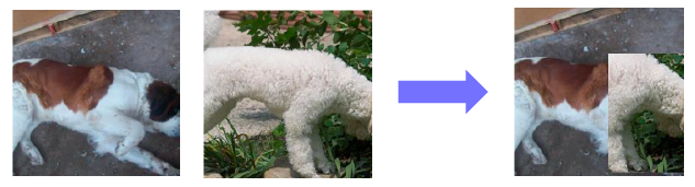
-
Generating new training image
-
Mixing both images and labels.
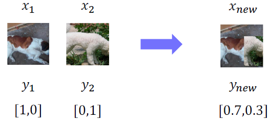
0.3이라는 값이 나오려면 어디를 참조해서 학습해야하는지 네트워크가 학습을 하게된다.
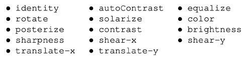
RandAugment
- Many augmentation methods exist. Hard to find best augmentations to apply.
- Automatically finding the best sequence of augmentations to apply.
- Random sample, apply, and evaluate augmentations.
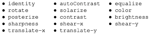
- Example of augmented images in RandAug
- Augmentation policy has two parameters
- Which augmentation to apply
- Magnitude of augementation to apply (how much to augment)
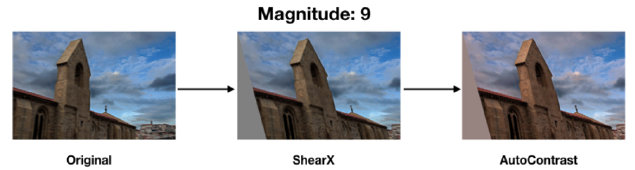
- Parameters used in the above example
- Which augmentation to apply : ‘ShearX’ & AutoContrast’
- Magnitude of augmentation to apply : 9
- Augmentation policy has two parameters
- Randomly testing augmentation policies
- Finding the best augmentation policy
- Sample a policy : Policy = {N augmentations to apply} by random sampling.
- Train with a sampled policy, and evaluate the accuracy.
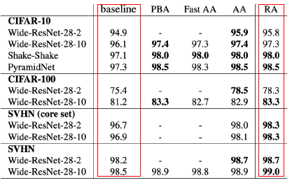
- Finding the best augmentation policy
- Augmentation helps model learning
- Higher test accuracy than training without augmentation.
Leveraging pre-trained information
Transfer learning
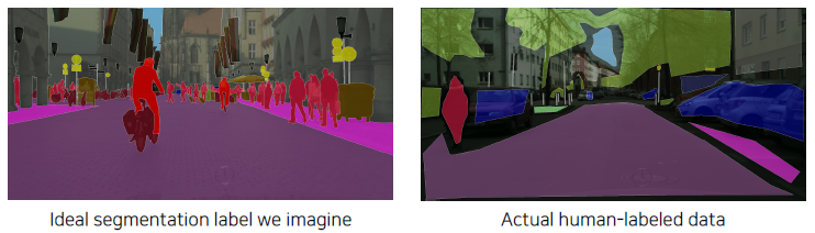
The high quality dataset is expensive and hard to obtain
- Supervised learning requires a very large scale dataset for training.
- Annotating data is very expensive, and its quality is not ensured.
- Transfer learning : A practical training method with a small dataset!
Benefits when using transfer learning.
- By transfer learning, we can easily adapt to a new task by leveraging pre trained knowledge (feature)!
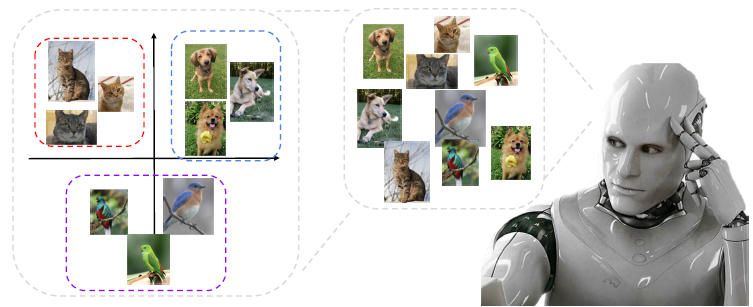
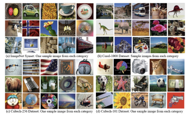
Motivational observation : Similar datasets share common information.
- E.g., 4 distinct datasets with similar images
- Knowledge learned from one dataset can be applied to other datasets!
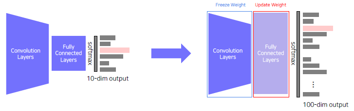
Approach 1 : Transfer knowledge from a pre trained task to a new task
- Given a model pre trained on a 10 class dataset,
- Chop off the final layer of the pre trained model, add and only re train a new FC layer.
- Extracted features preserve all the knowledge from pre training.
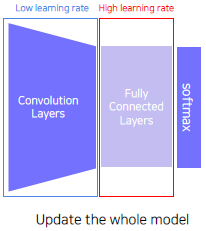
Approach 2 : Fine tuning the whole model
- Given a model pre trained on a dataset
- Replace the final layer of the pre trained model to a new one, and re train the whole model.
- Set learning rates differently.
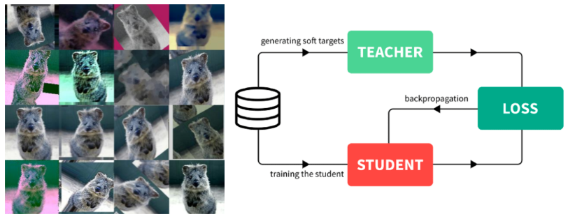
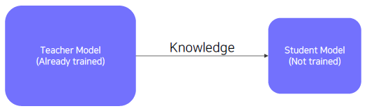
Knowledge distillation
Passing what model learned to 'another' smaller model (Teacher student learning)
- 'Distillate' knowledge of a trained model into another smaller model.
- Used for model compression. (Mimicking what a larger model knows)
- Also, used for pseudo labeling. (Generating pseudo labels for an unlabeled dataset)
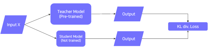
Teacher student network structure.
- The student network learns what the teacher network knows.
- The student network mimics outputs of the teacher network.
- Unsupervised learning, since training can be done only with unlabeled data.
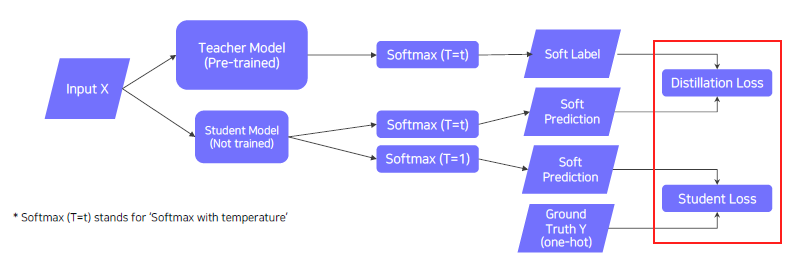
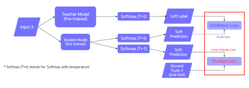
Knowledge distillation
- When labeled data is available, can leverage labeled data for training (Student Loss)
- Distillation loss to 'predict similar outputs with the teacher model'
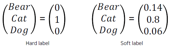
Hard label vs Soft label
- Hard label (One hot vector)
- Typically obtained from the dataset
- Indicates whether a class is 'true answer' or not
- Soft label
- Typicall output of the model (=inference result)
- Regard it as "knowledge". Useful to observe how the model thinks
Softmax with temperature()
- Softmax with temperature : controls difference in output between small & large input values
- A large 𝑇 smoothens large input value differences.
- Useful to synchronize the student and teacher models' outputs
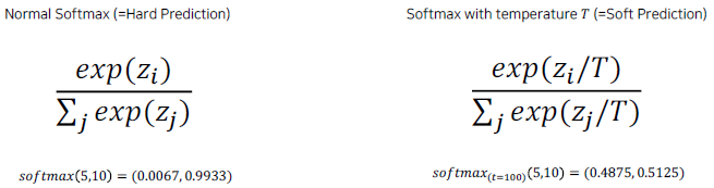
입력값을 temperature T라는 큰 값으로 나누어 주어 출력을 좀 더 부드럽게 해준다. 0 또는 1 이라기 보다는 전체 softmax의 크고 작은 지식들을 표현하는데 더 유용하다.
- Semantic information is not considered in distillation
Teacher의 각 특징들이 주는 정보가 중요하기 보다는 그 행동을 따라하는 것에 초점을 둔다.
Intuition about distillation loss and student loss
- Distillation Loss
- KLdiv(Soft label, Soft prediction)
- Loss = difference between the teacher and student network's inference
- Learn what teacher network knows by mimicking
- Student Loss
- CrossEntropy. (Hard label, Soft prediction)
- Loss = difference between the student network's inference and true label.
- Learn the 'right answer'.
Loss functions in knowledge distillation
- Weighted sum of "Distillation loss" and "Student loss"
Leveraging unlabeled dataset for training
Semi-supervised learning
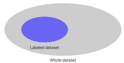
There are lots of unlabeled data
- Typically, only a small portion of data is labeled.
- Is there any way to learn from unlabeled data?
- Semi supervised learning : Unsupervised (No label) + Fully Supervised (fully labeled)
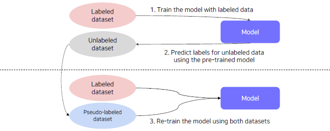
Semi supervised learning with pseudo labeling.
- Pseudo labeling unlabeled data using a pre trained model, then use for training.
Self-training
Recap : Data efficient learning methods so far
-
Data Augmentation
- Augment a dataset to make the dataset closer to real data distribution
-
Knowledge distillation
- Train a student network to imitate a teacher network
- Transfer the teacher network’s knowledge to the student network
-
Semi supervised learning (Pseudo label based method)
- Pseudo label an unlabeled dataset using a pre trained model, then use for training
- Leveraging an unlabeled dataset for training!
Self-training
- Augmentation + Teacher Student networks + semi supervised learning
- SOTA ImageNet classification, 2019
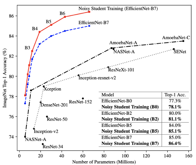
Self-training with noisy student
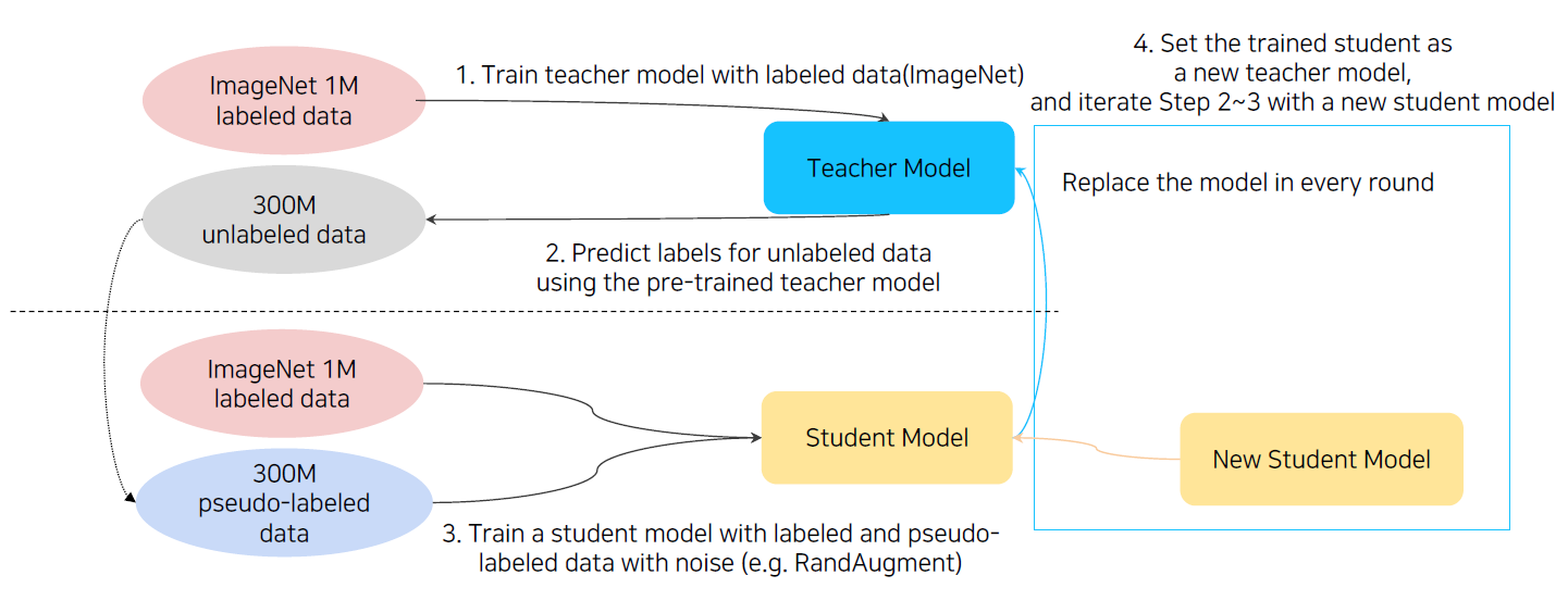
Iteratively training noisy student network using teacher network.
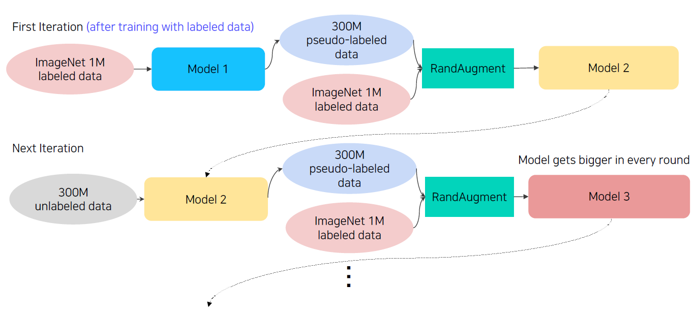
Brief overview of self-training
- Train initial teacher model with labeled data.
- Pseudo label unlabeled data using teacher model.
- Train student model with both lableled and unlabeled data with augmentation.
- Set the student model as a new teacher, and set new model (bigger) as a new student.
- Repeat 2~4 with new teacher/student models.
