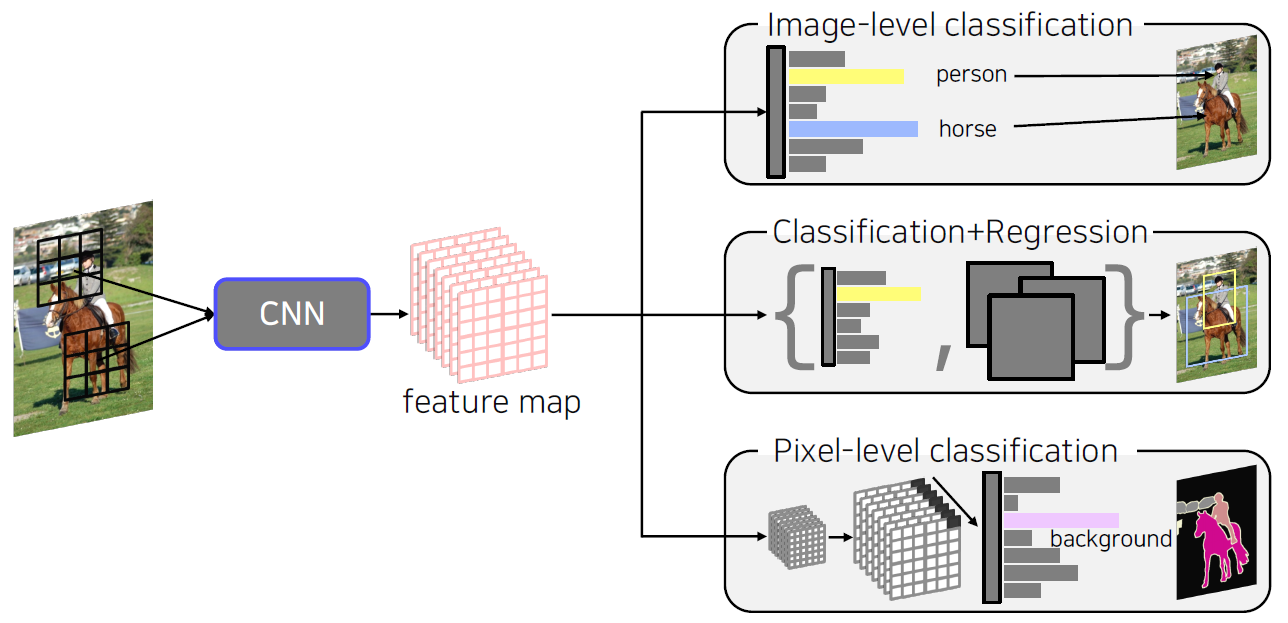
Image classification

Problems with deeper layers

Going deeper with convolutions

The neural network is getting deeper and wider.

• Deeper networks learn more powerful features, because of
  • Larger receptive fields
  • More capacity and non-linearity
• But, getting deeper and deeper always works better?

Hard to optimize

Deeper networks are harder to optimize.

• Gradient vanishing / exploding
• Computationally complex
• Degradation problem
  Increasing the depth of a network leads to a decrease in performance on both test and training data.

---

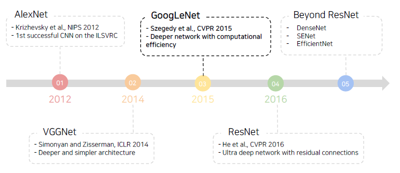
CNN architectures for image classification

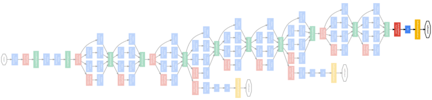
GoogLeNet

Inception module

• Apply multiple filter operations on input activation from the previous layer:
  • 1x1, 3x3, 5x5 convolution filters
  • 3x3 pooling operation
• Concatenate all filter outputs together along the channel axis.

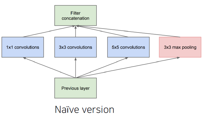
• The increased network size increases the use of computational resources.
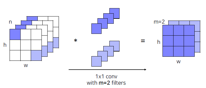
• Use 1x1 convolutions!

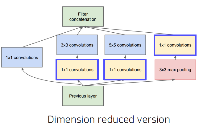
• Use 1x1 convolutions as ”bottleneck” layers that reduce the number of channels.

Overall architecture

• Stem network: vanilla convolution networks.

• Stacked inception modules

• Auxiliary classifiers

• The vanishing gradient problem is dealt with by the auxiliary classifier.
• Injecting additional gradients into lower layers.
• Used only during training, removed at testing time.

층이 깊어지면 gradient vanishing 현상이 일어날 수 있기 때문에 중간 중간 결과에 task를 두고 gradient 를 주사기처럼 주입한다. 각 classifier는 마지막 층의 classifier와 동일하다.

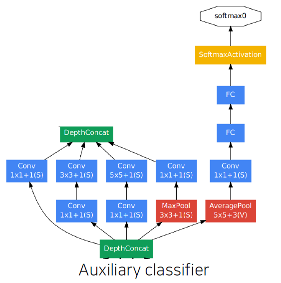
• Classifier ouput (a single FC layer)

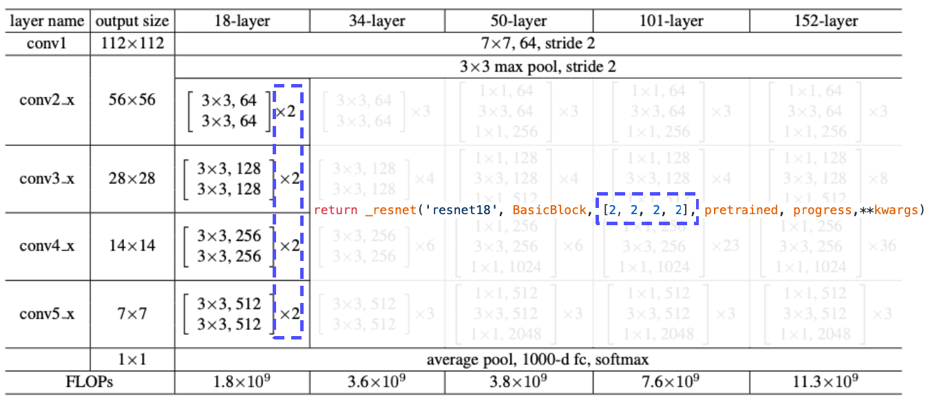
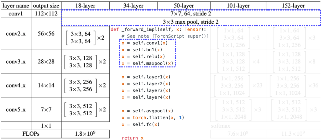
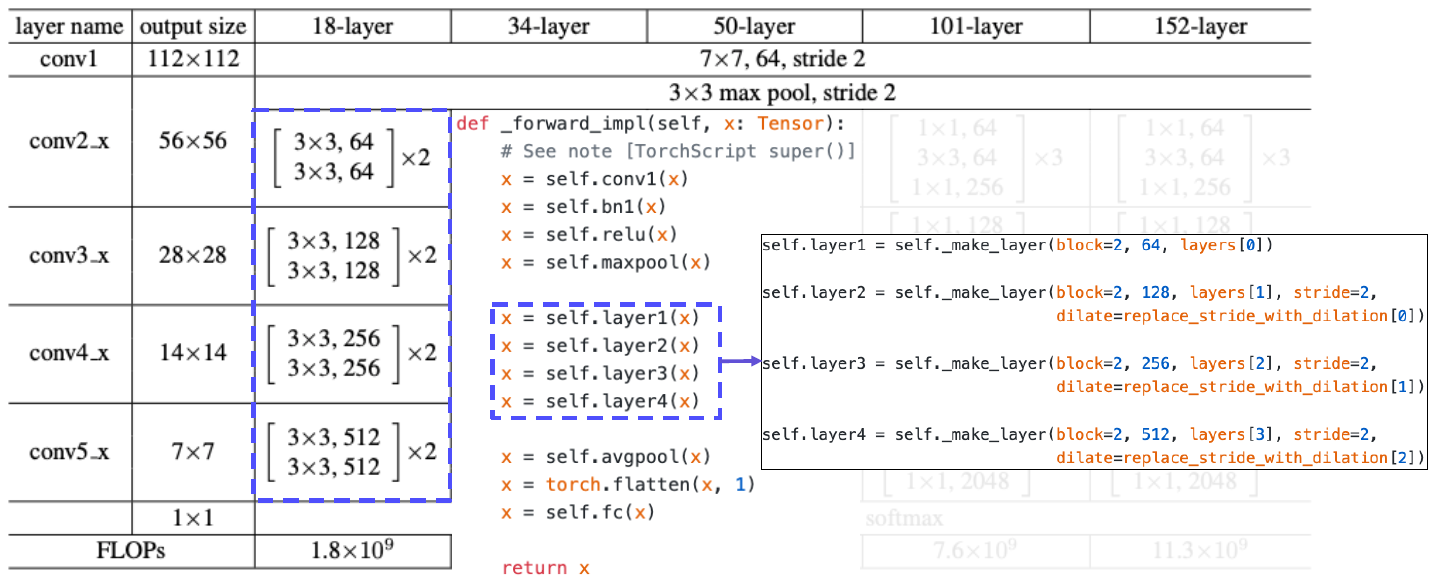
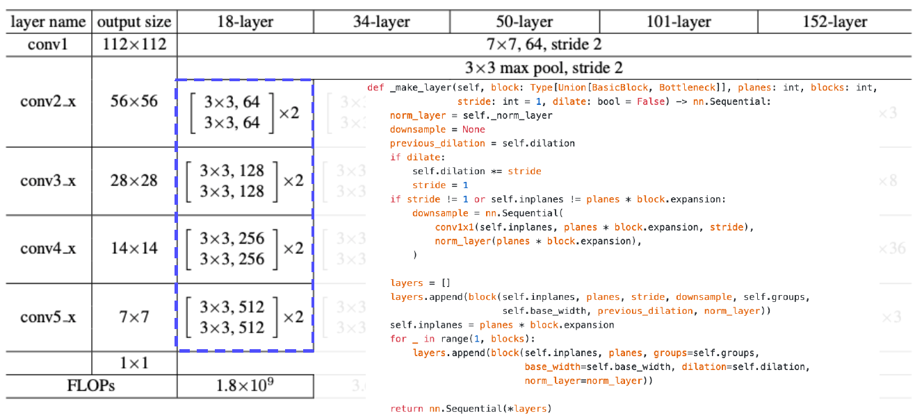
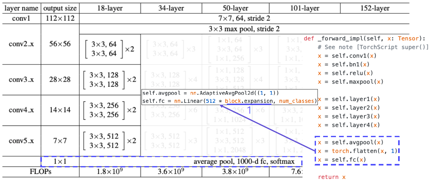
ResNet

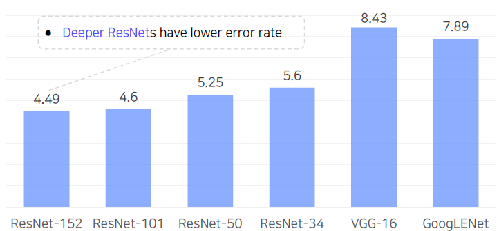
Top-5 validation error on the ImageNet

Revolutions of depth

• Building ultra-deeper than any other networks
• What makes it hard to build a very deep architecture?

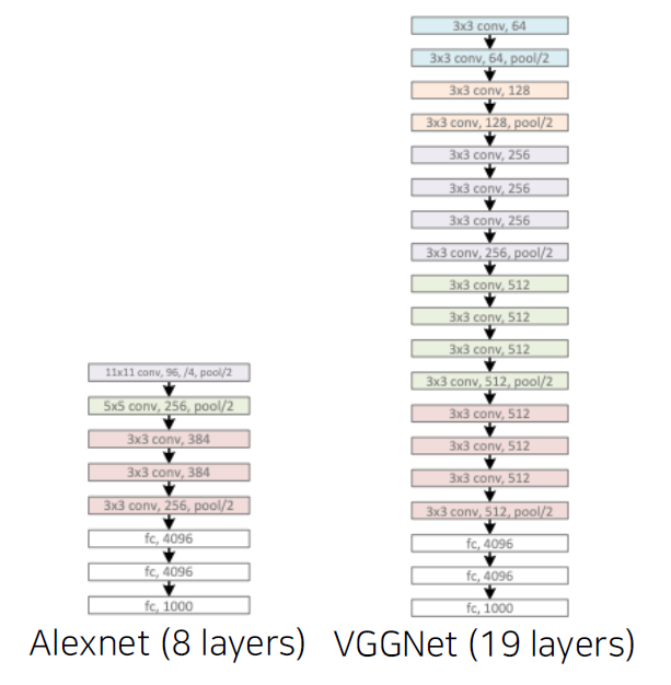
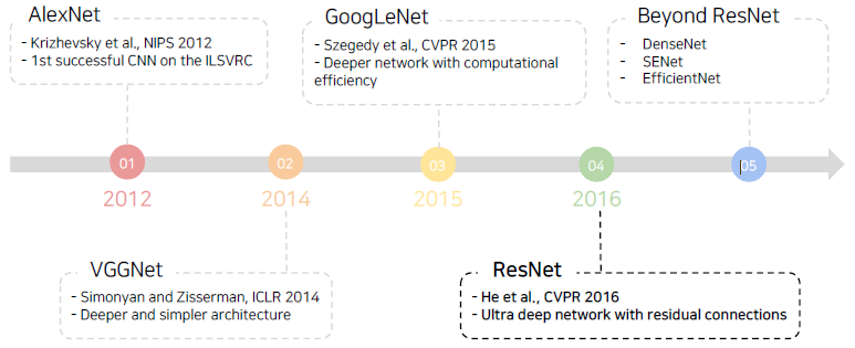
AlexNet (8 layers)

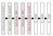
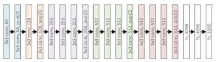
VGGNet (19 layers)

ResNet (152 layers)

Degradation problem

• As the network depth increases, accuracy gets saturated → degrade rapidly

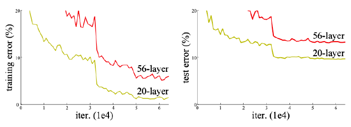
만약 overfitting이 일어난다면 traning error에 대해서 56-layer가 20-layer 보다 더 성능이 좋아야 하는데 그렇지 않았다. 즉, 층을 깊이 쌓아서 생기는 문제는 overfitting problem이 아니고 gradient vanishing과 explosion에 발생하는 degradation problem이다.

Hypothesis

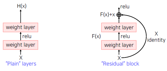
• Plain layer: As the layers get deeper, it is hard to learn good $H(x)$ directly.
• Residual block: Instead, we learn residual.
  • Target function : $H(x)=F(x)+x$
  • Residual function : $F(x)=H(x)-x$

A solution: Shortcut connection

• Use layers to fit a residual mapping instead of directly fitting a desired underlying mapping.
• The vanishing gradient problem is solved by shortcut connection.
• Don’t just stack layers up, instead use shortcut connection!

Analysis of residual connection

• During training, gradients are mainly from relatively shorter paths.
• Residual networks have $O(2^n)$ implicit paths connecting input and output, and adding a block doubles the number of paths.

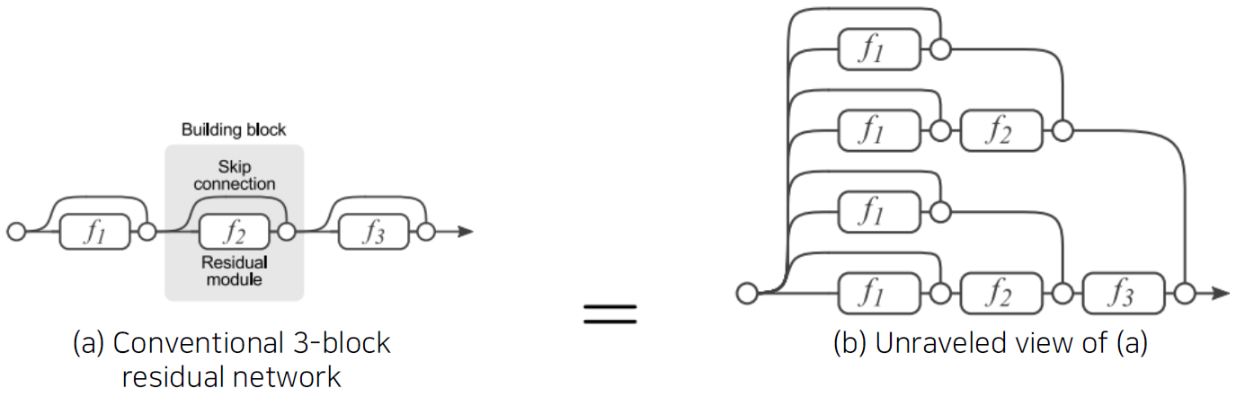
층이 깊어질수록 graident가 전달되는 경로의 수가 커지기 때문에 바로 가는 path를 포함하여 중간을 모두 거쳐가는 path까지 다양한 경로를 통해서 굉장히 복잡한 mapping을 학습할 수 있다.

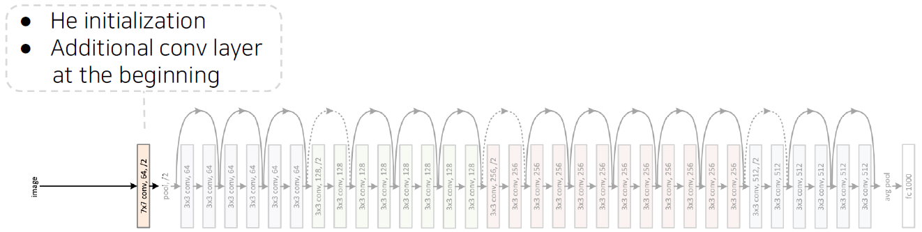
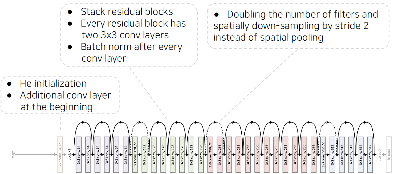
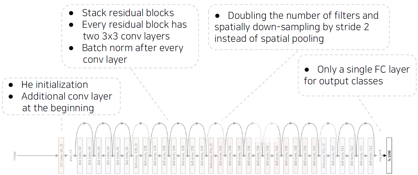
Overall architecture

PyTorch code for ResNet

Beyond ResNets

• DenseNet
  • In ResNet, we added the input and the output of the layer element-wisely.
  • In the Dense blocks, every output of each layer is concatenated along the channel axis.
    • Alleviate vanishing gradient problem
    • Strengthen feature propagation
    • Encourage the reuse of features

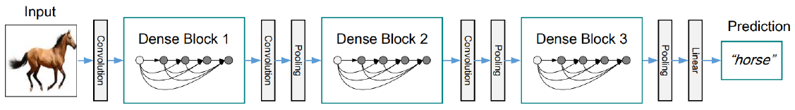
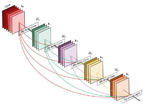
ResNet은 신호를 합치지만 DenseNet은 신호를 그대로 concat해서 원래의 신호를 보존한다. 채널이 계속 늘어나서 메모리 사용이나 계산 복잡도가 증가한다.

• SENet
  • Attention across channels.
  • Recalibrates channel-wise responses by modeling interdependencies between channels.
  • Squeeze and excitation operations.
    • Squeeze: capturing distributions of channel-wise responses by global average pooling.
    • Excitation: gating channels by channel-wise attention weights obtained by a FC layer.

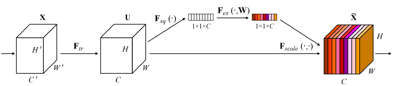
conv에서 나온 결과값을 vector화(channel별로 average pooling)해서 주목해야 하는 channel에 attention을 주고, 이를 이용하여 원래 채널의 값들을 re-scaling한다.

• EfficientNet
  • Building deep, wide, and high resolution networks in an efficient way.

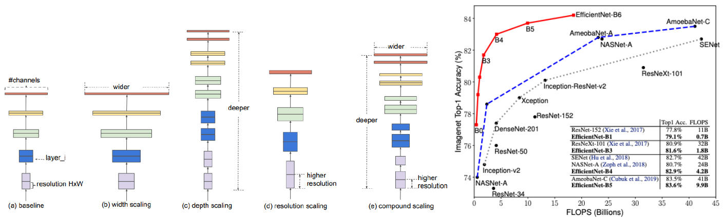
width, depth, resolution scaling을 compound해서 사용한다.

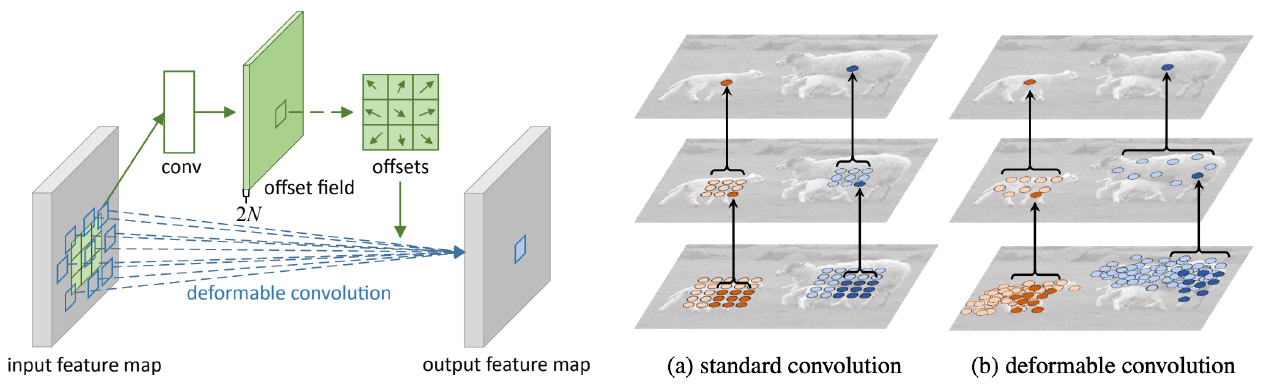
• Deformable convolution
  • 2D spatial offset prediction for irregular convolution.
  • Irregular grid sampling with 2D spatial offsets.
  • Implemented by standard CNN and grid sampling with 2D offsets.

---

Summary of image classification

Summary of image classification

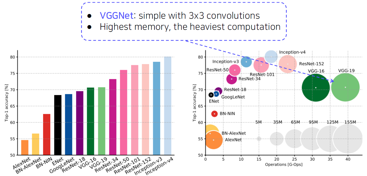
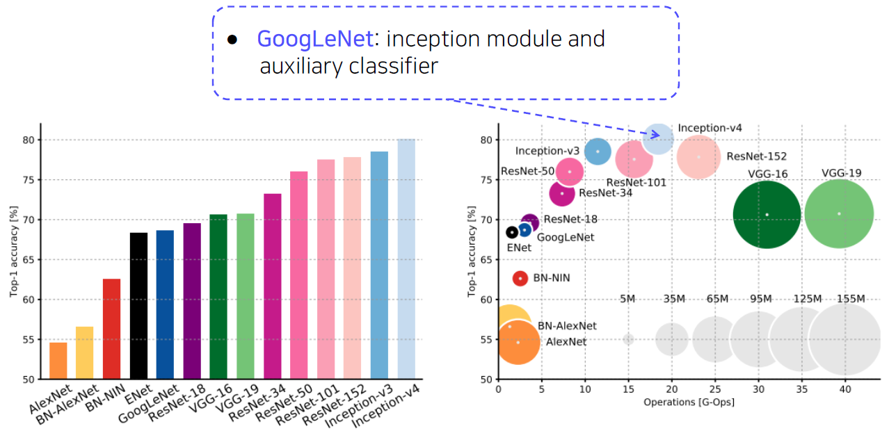
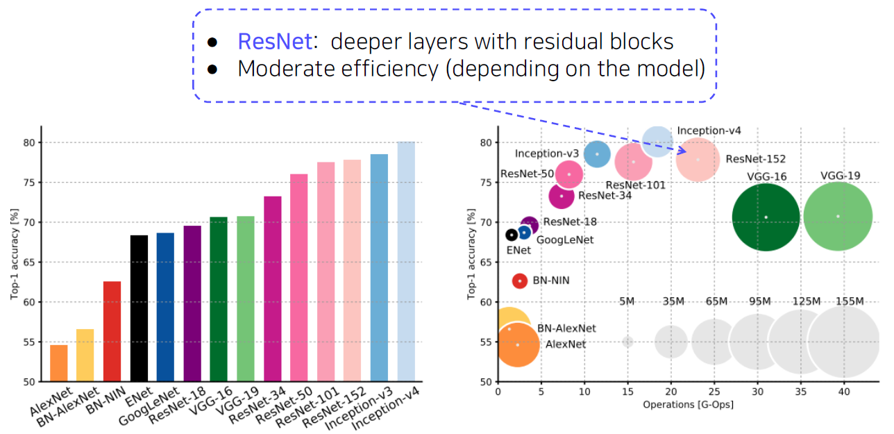
CNN backbones

Simple but powerful backbone model

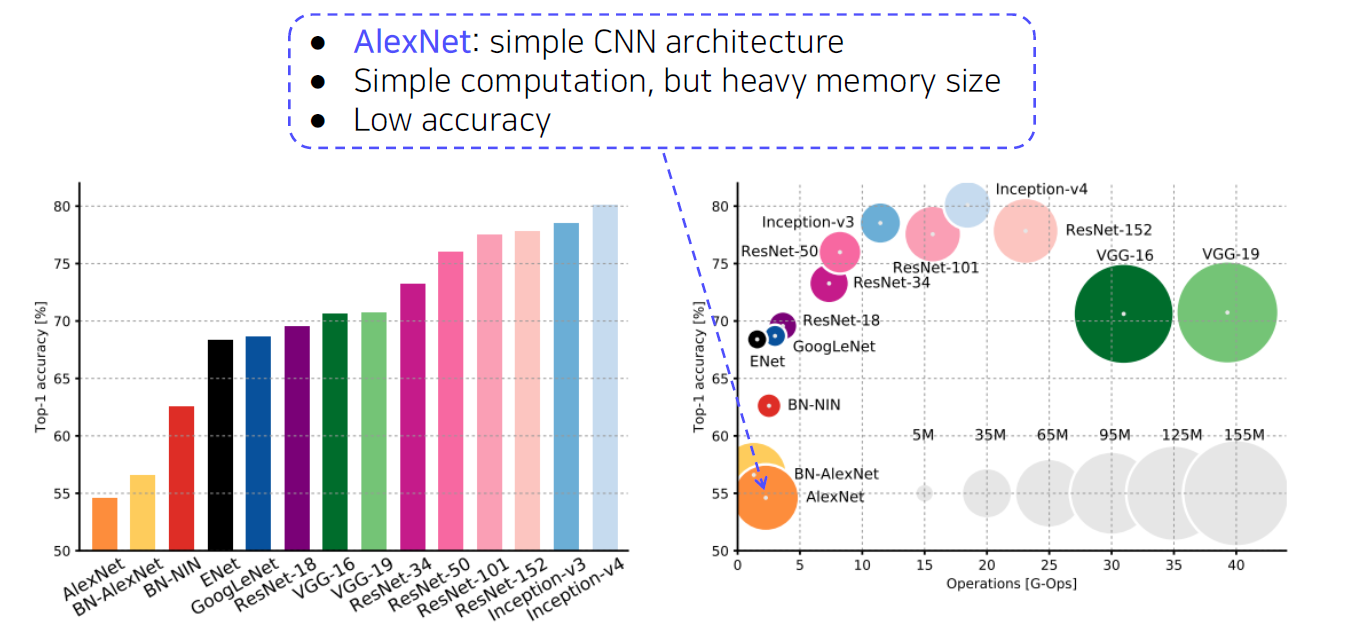
• GoogLeNet is the most efficient CNN model out of {AlexNet, VGG, ResNet}.
• But, it is complicated to use.

• Instead, VGGNet and ResNet are typically used as a backbone model for many tasks.
• Constructed with simple 3x3 conv layers.

Semantic segmentation

Semantic segmentation

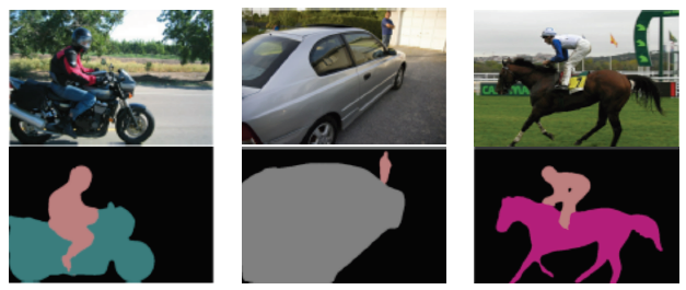
What is semantic segmentation?

Semantic segmentation

• Classify each pixel of an image into a category.
• Don’t care about instances. Only care about semantic category.

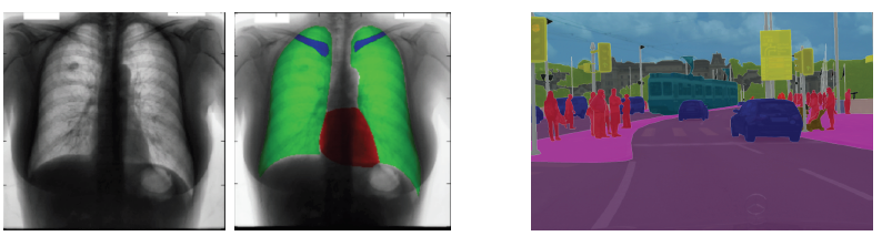
Where can semantic segmentation be applied to?

Applications

• Medical images
• Autonomous driving
• Computational photography

---

Semantic segmentation architectures

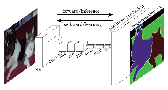
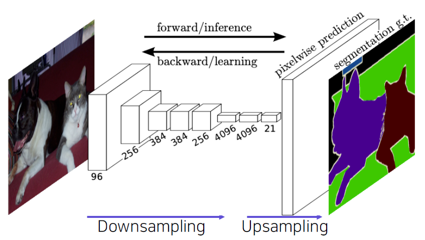
Fully Convolutional Networks (FCN)

Fully Convolutional Networks

• The first end-to-end architecture for semantic segmentation.
• Take an image of an arbitrary size as input, and output a segmentation map of the corresponding size to the input.

Fully connected vs Fully convolutional

• Fully connected layer: Output a fixed dimensional vector and discard spatial coordinates.
• Fully convolutional layer: Output a classification map which has spatial coordinates.

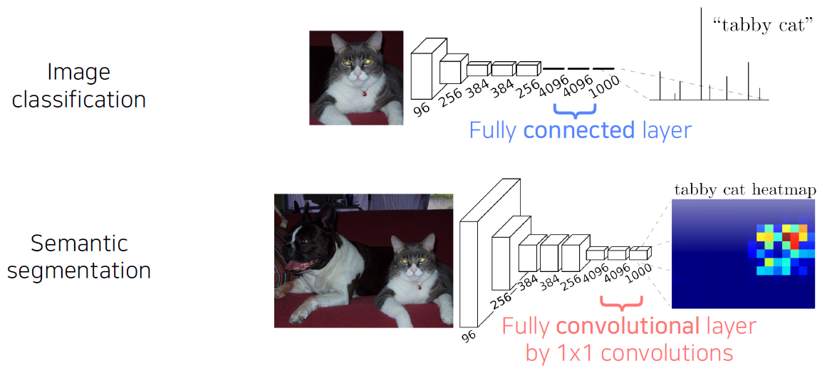
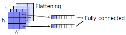
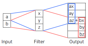
Interpreting fully connected layers as 1x1 convolutions.

• A fully connected layer classifies a single feature vector.

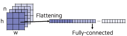
channel별로 하는 Flattening은 spatial 정보가 사라지게 된다.

따라서 channel축으로 Flattening을 진행한다.

• A 1x1 convolution layer classifies every feature vector of the convolutional feature map.

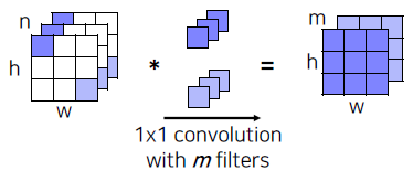
• A 1x1 convolution layer classifies every feature vector of the convolutional feature map.
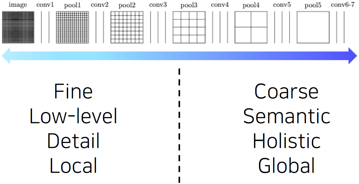
• Limitation: Predicted score map is in a very low-resolution.
• Why?
  • For having a large receptive field, several spatial pooling layers are deployed.
    pooling layer와 stride는 더 큰 receptive field size를 갖기 위해 쓰이고 이로 인해 해상도가 낮아지게 된다.
• Solution: Enlarge the score map by upsampling!

Upsampling

• The size of the input image is reduced to a smaller feature map.
• Upsample to the size of input image.

• Upsampling is used to resize a small activation map to the size of the input image.
  • Unpooling
  • Transposed convolution
  • Upsample and convolution

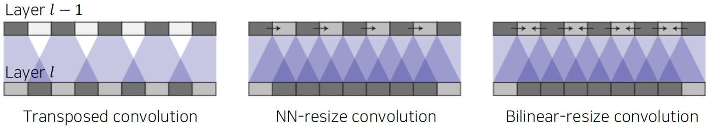
Transposed convolution

Transposed convolutions work by swapping the forward and backward passes of convolution.

적절한 conv 사이즈와 stride를 넣지 않으면 위 그림처럼 $az+bx$의 중복되는 부분이 생기게 된다.

Problems with transposed convolution.

• Checkerboard artifacts due to uneven overlaps

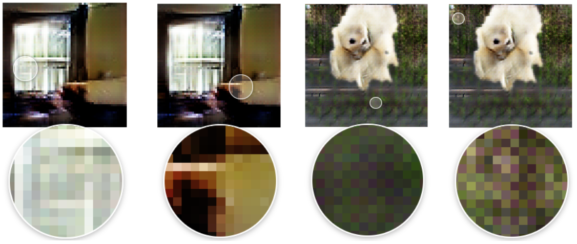
그 결과 위 그림처럼 얼룩진 패턴이 나타나게 된다.

Better approaches for upsampling.

• Avoid overlap issues in transposed convolution.
• Decompose into spatial upsampling and feature convolution.
  • {Nearest-neighbor (NN), Bilinear} interpolation followed by convolution.

Back to FCN

Adding skip connections for enlarging the score map.

Semantic segmentation을 하려면 낮은 layer가 갖고 있는 국지적인 정보와 높은 layer가 갖고 있는 전체적인 맥락 정보를 모두 포함해야 한다. 각 pixel별로 의미를 파악해야 하고, 영상 전체를 바라보면서 현재 pixel이 물체의 경계선 안쪽에 해당하는지 바깥쪽에 해당하는지 파악할 수 있어야 한다.

• Integrates activations from lower layers into prediction.
• Preseves higher spatial resolution.
• Captures lower-level semantics at the same time.

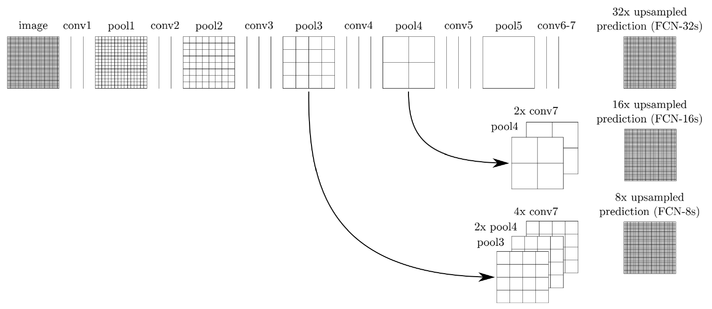
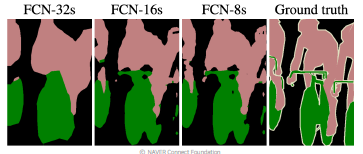
이때 사용되는 8, 16, 32의 넘버링은 정보를 얼마나 upsampling 한 건지 나타낸다. 32는 제일 마지막 단 layer의 정보만을 갖고 원래의 input size로 upsampling을 하기 때문에 $2^5$ upsampling을 한다. 16은 그 전 layer 하나를 더 포함해서 upsampling을 해서 $2^4$ 만큼만 upsampling한다.

Features of FCN

• Faster

  • The end-to-end architecture that does not depend on other hand-crafted components.

• Accurate

  • Feature representation and classifiers are jointly optimized.

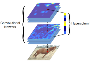
Hypercolumns for object segmentation

Fully convolutional networks

• CNN layers typically use the output of the last layer as feature representation.

  • Too coarse spatially

• Hypercolumn at a pixel is a stacked vector of all CNN units on that pixel

  • Fine localized information is extracted from earlier layers.
  • Coarse semantic information is extracted from latter layers.

Overall architecture

• (Concurrent work) Very similar to FCN.
• Difference: Apply to each bounding box.

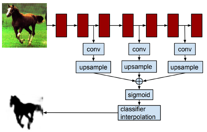
hypercolumn 방식은 물체에 bounding box를 구하는 외부 알고리즘(신경망이 아님)을 이용했기에 end-to-end 방식이 아니다.

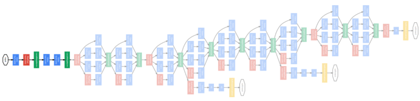
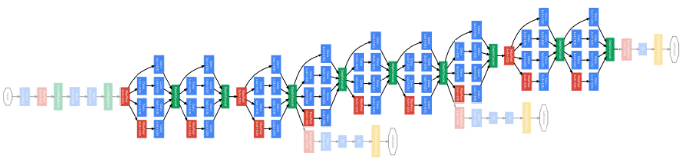
U-Net

• Built upon "fully convolutional networks".
  • Share the same FCN property.
    
    
• Predict a dense map by concatenating feature maps from contracting path.
  • Similar to/skip/connections/in/FCN.
    
    
• Yield more precise segmentations.

Overall architecture

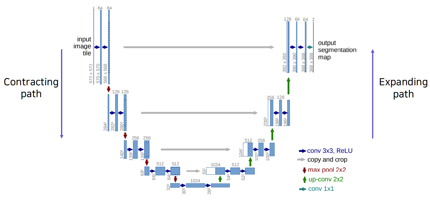
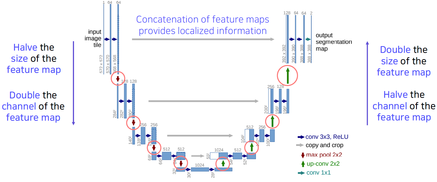
• Contracting Path
  • Repeatedly applying 3x3 convolutions.
  • Doubling the number of feature channels.
  • Being used to capture holistic context.
    
    
• Expanding Path
  • Repeatedly applying 2x2 convolutions.
  • Halving the number of feature channels.
  • Concatenating the corresponding feature maps from the contracting path.

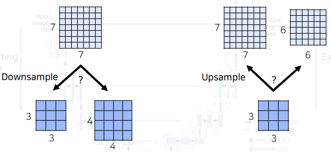
What if the spatial size of the feature map is an odd number?

An even number is required for input and feature sizes.

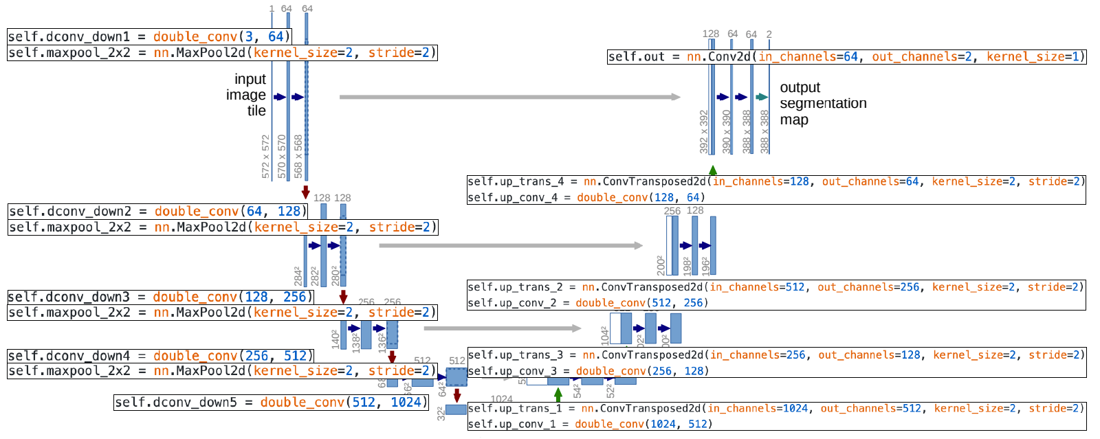
PyTorch code for U-Net

def double_conv(in_channels, out_channels):
    return nn.Sequential(
        nn.Conv2d(in_channels, out_channels, 3),
        nn.ReLU(inplace = True),
        nn.Conv2d(out_channels, out_channels, 3),
        nn.ReLU(inplace = True)
    )

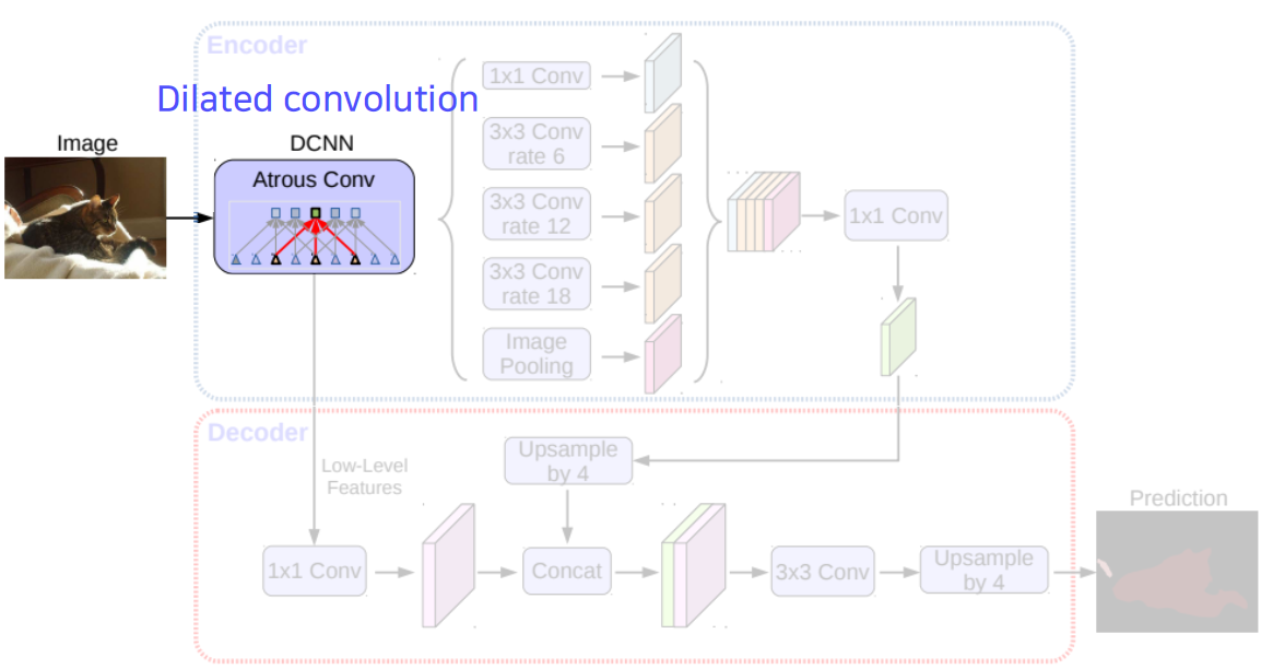
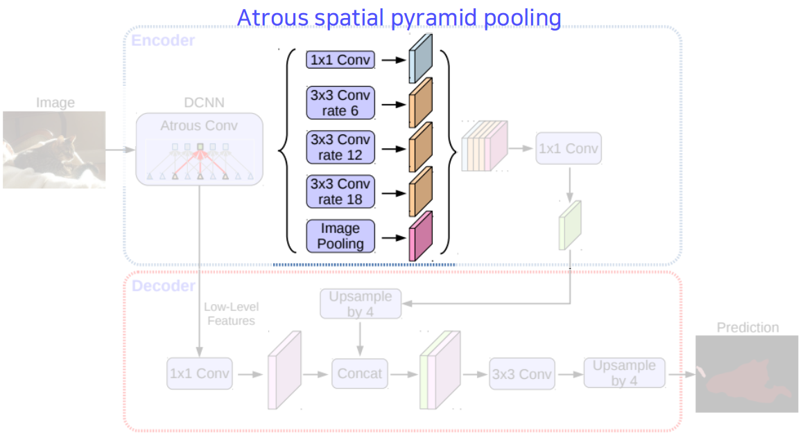
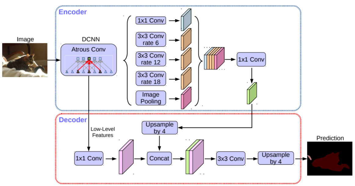
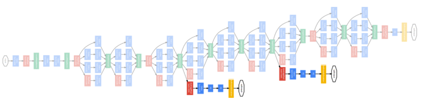
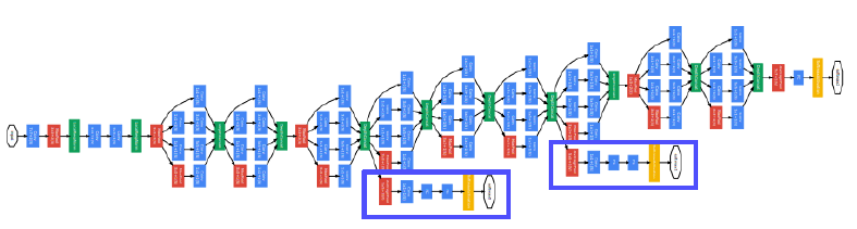
DeepLab

• DeepLab v1 (2015)
  Semantic Image Segmentation with Deep Convolutional Nets and Fully Connected CRFs. ICLR 2015.
  
  
• DeepLab v2 (2017)
  DeepLab: Semantic Image Segmentation with Deep Convolutional Nets, Atrous Convolution, and Fully Connected CRFs. TPAMI 2017.
  
  
• DeepLab v3 (2017)
  Rethinking Atrous Convolution for Semantic Image Segmentation. arXiv 2017.
  
  
• DeepLab v3+ (2018)
  Encoder-Decoder with Atrous Separable Convolution for Semantic Image Segmentation. ECCV 2018

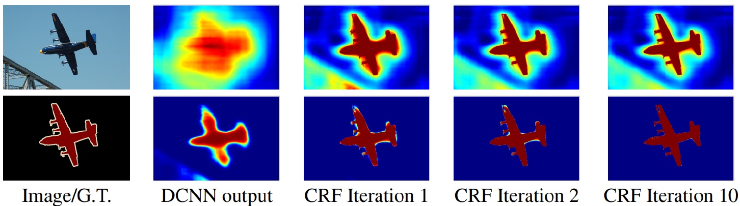
Conditional Random Fields (CRFs)

• CRF post-processes a segmentation map to be refined to follow image boundaries.
• 1st row: score map (before softmax) / 2nd row : belief map (after softmax)

Dilated convolution

• Atrous convolution.
• Inflate the kernel by inserting spaces between the kernel element (Dilation factor).
• Enable exponential expansion of the receptive field.

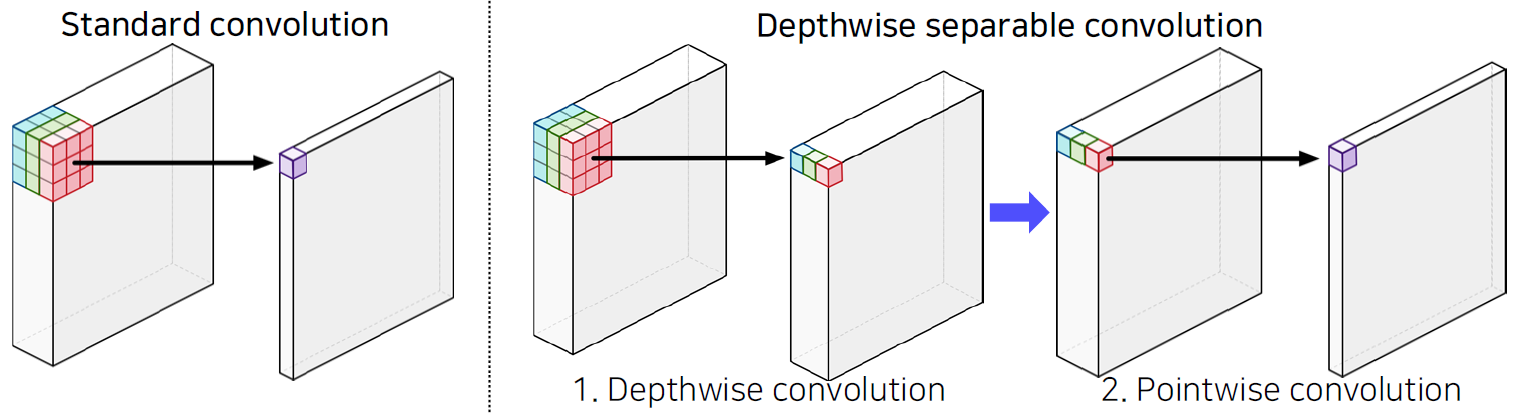
Depthwise separable convolution (proposed by Howard et al.)

• No. parameters
  • Standard conv: $D_K^2MND_F^2$
    차원수 관점에서 보면 2+1+1+2 = 6차원
    
    
  • Depthwise separable conv: $D_K^2MD_F^2 + MND_F^2$
    차원수 관점에서 보면 2+1+2, 1+1+2 최고 차원이 5차원

Deeplab v3+