Ai tech Day6

Lee·2021년 1월 25일

Numerical Python (numpy)

파이썬의 고성능 과학 계산용 패키지

numpy

Numerical Python

Array 연산의 표준
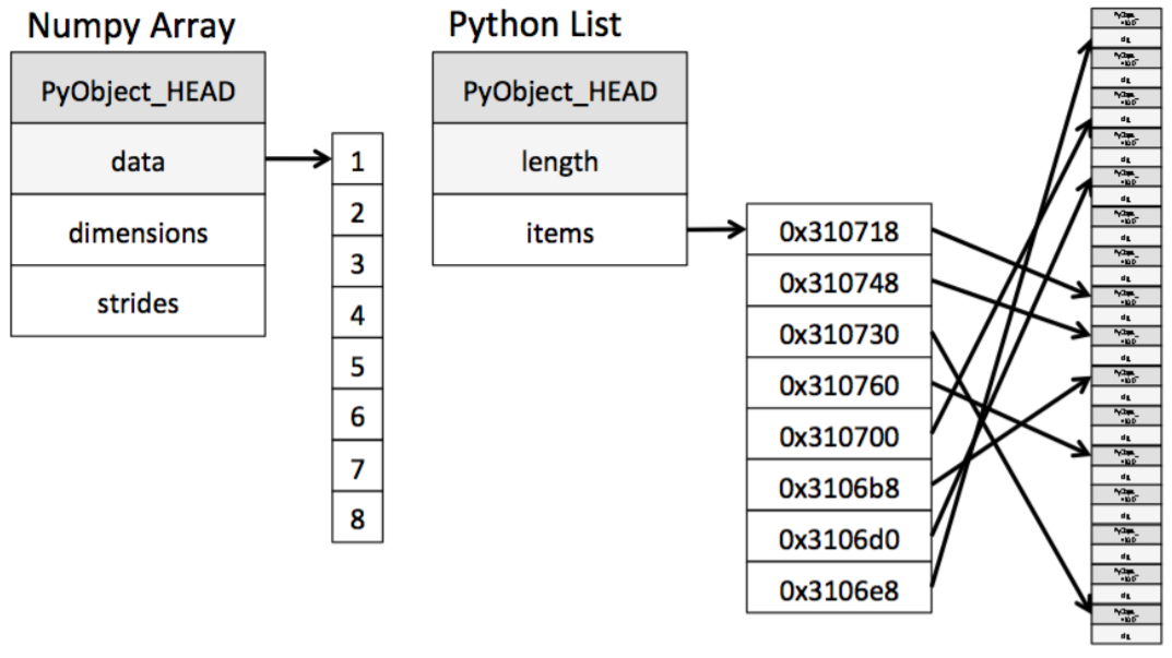
일반 List에 비해 빠르고, 메모리 효율적
반복문 없이 데이터 배열에 대한 처리를 지원한다.
선형대수와 관련된 다양한 기능을 제공한다.
C, C++, 포트란 등의 언어와 통합 가능하다.
numpy install
Windows 환경에선 conda로 패키지 관리 필요
```
conda install numpy
```

ndarray

import
import numpy as np
- numpy의 호출 방법
- 일반적으로 np라는 alias(별칭)을 이용해서 호출한다.
array creation
numpy는 np.array 함수를 활용해 배열을 생성한다. (ndarray 객체)
- numpy는 하나의 데이터 type만 배열에 넣을 수 있다.
- Dynamic typing not supproted (List와 가장 큰 차이점)
- C의 Array를 사용하여 배열을 생성한다.

test_array = np.array([1, 4, 5, 8], float)
print(test_array)
type(test_array[3])

test_array = np.array([1, 4, 5, 8], float)
test_array
# array([1., 4., 5., 8.])

type(test_array[3])
# numpy.float64

shape: numpy array의 dimension 구성을 반환한다.

matrix = [[1, 2, 5, 8], [1, 2, 5, 8], [1, 2, 5, 8]]
np.array(matrix, int).shape
# (3, 4)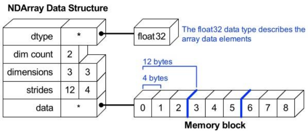
# Tuple shape

dtype
ndarray의 single element가 가지는 data type을 반환한다.
각 element가 차지하는 momory의 크기가 결정된다. (not dynamic typing)

test_array = np.array([1, 4, 5, "8"], float) # String Type의 데이터를 입력해도
print(test_array)
print(type(test_array[3])) # Float Type으로 자동 형변환을 실시
print(test_array.dtype) # Array(배열) 전체의 데이터 Type을 반환함
print(test_array.shape) # Array(배열) 의 shape을 반환함

array의 RANK에 따라 불리는 이름이 존재

Rank Name Example
0 scalar 7
1 vector [10, 10]
2 matrix [[10, 10], [15, 15]]
3 3-tensor [[[1, 5, 9], [2, 6, 10]], [[3, 7, 11], [4, 8, 12]]]
n n-tensor
ndim
number of dimensions
size
data의 개수

Rank	Name	Example
0	scalar	7
1	vector	[10, 10]
2	matrix	[[10, 10], [15, 15]]
3	3-tensor	[[[1, 5, 9], [2, 6, 10]], [[3, 7, 11], [4, 8, 12]]]
n	n-tensor

nbytes
ndarray object의 메모리 크기를 반환한다.

np.array([[1, 2, 3], [4.5, '5', '6']], dtype = np.float32).nbytes
# 24 (32bits = 4bytes -> 6 * 4bytes)

Handling shape

reshape

Array의 shape의 크기를 변경한다. (element의 갯수는 동일)

test_matrix = [[1, 2, 3, 4], [1, 2, 5, 8]]
np.array(test_matrix).shape
# (2, 4)

np.array(test_matrix).reshape(8,)
# array([1, 2, 3, 4, 1, 2, 5, 8])

np.array(test_matrix).reshape(8,).shape
# (8,)

# -1: size를 기반으로 row 개수 선정
np.array(test_matrix).reshape(-1, 2).shape
# (4, 2)

flatten

다차원 array를 1차원 array로 변환 ( (2, 2, 4) -> (16,) )

test_matrix = [[[1, 2, 3, 4], [1, 2, 5, 8]], [[1, 2, 3, 4], [1, 2, 5, 8]]]
np.array(test_matrix).flatten()
# array([1, 2, 3, 4, 1, 2, 5, 8, 1, 2, 3, 4, 1, 2, 5, 8])

indexing & slicing

indexing

list와 달리 이차원 배열에서 [0, 0] 표기법을 제공한다.

matrix일 경우 앞은 row 뒤는 column 을 의미한다.

a = np.array([[1, 2, 3], [4.5, 5, 6]], int)
print(a)
print(a[0,0]) # Two dimensional array representation #1
print(a[0][0]) # Two dimensional array representation #2

a[0,0] = 12 # Matrix 0,0 에 12 할당
print(a)
a[0][0] = 5 # Matrix 0,0 에 12 할당
print(a)

slicing

list와 달리 행과 열 부분을 나눠서 slicing이 가능하다.

matrix의 부분 집합을 추출할 때 유용하다.

a = np.array([[1, 2, 3, 4, 5], [6, 7, 8, 9, 10]], int)
a[:,2:] # 전체 Row의 2열 이상
a[1,1:3] # 1 Row의 1열 ~ 2열
a[1:3] # 1 Row ~ 2Row의 전체

creation function

arange

array의 범위를 지정하여 값의 list를 생성하는 명령어

np.arange(30) # range: list의 range와 같은 효과, intger로 0부터 29까지 배열 추출
#array([ 0,  1,  2,  3,  4,  5,  6,  7,  8,  9, 10, 11, 12, 13, 14, 15, 16, 17, 18, 19, 20, 21, 22, 23, 24, 25, 26, 27, 28, 29])

np.arange(0, 5, 0.5) # floating point도 표시 가능함
# array([0. , 0.5, 1. , 1.5, 2. , 2.5, 3. , 3.5, 4. , 4.5])

np.arange(30).reshape(5, 6)
# array([[ 0,  1,  2,  3,  4,  5],
#       [ 6,  7,  8,  9, 10, 11],
#       [12, 13, 14, 15, 16, 17],
#       [18, 19, 20, 21, 22, 23],
#       [24, 25, 26, 27, 28, 29]])

zeros

0으로 가득찬 ndarray 생성

np.zeros(shape, dtype, order)

np.zeros(shape = (10,), dtype = np.int8) # 10 - zero vector 생성
# array([0, 0, 0, 0, 0, 0, 0, 0, 0, 0], dtype=int8)

np.zeros((2, 5)) # 2 by 5 - zero matrix 생성
# array([[0., 0., 0., 0., 0.],
#        [0., 0., 0., 0., 0.]])

ones

1로 가득찬 ndarray 생성

np.ones(shape = (10,), dtype = np.int8)
# array([1, 1, 1, 1, 1, 1, 1, 1, 1, 1], dtype=int8)

np.ones((2, 5))
# array([[1., 1., 1., 1., 1.],
#        [1., 1., 1., 1., 1.]])

empty

shape만 주어지고 비어있는 ndarray 생성 (memory initialization 이 되지 않음)

initialization 이 되지 않아 생성 속도가 빠르다.

np.empty(shape = (10,), dtype = np.int8)
np.empty((3, 5))

something_like

기존 ndarray의 shape 크기 만큼 1, 0 또는 empty array를 반환

test_matrix = np.arange(30).reshape(5, 6)
np.ones_like(test_matrix)
# array([[1, 1, 1, 1, 1, 1],
#       [1, 1, 1, 1, 1, 1],
#       [1, 1, 1, 1, 1, 1],
#       [1, 1, 1, 1, 1, 1],
#       [1, 1, 1, 1, 1, 1]])

identity

단위 행렬(i 행렬)을 생성

np.identity(n = 3, dtype = np.int8)
# array([[1, 0, 0],
#        [0, 1, 0],
#        [0, 0, 1]], dtype=int8)

np.identity(5)
# array([[1., 0., 0., 0., 0.],
#        [0., 1., 0., 0., 0.],
#        [0., 0., 1., 0., 0.],
#        [0., 0., 0., 1., 0.],
#        [0., 0., 0., 0., 1.]])

eye

대각선이 1인 행렬

k 값으로 시작 index의 변경이 가능하다.
(k > 0 이면 column의 index, k < 0 이면 row의 index)

np.eye(3)
# array([[1., 0., 0.],
#        [0., 1., 0.],
#        [0., 0., 1.]])

np.eye(3, 5, k = 2)
# array([[0., 0., 1., 0., 0.],
#        [0., 0., 0., 1., 0.],
#        [0., 0., 0., 0., 1.]])

np.eye(N = 3, M = 5, dtype = np.int8)
# array([[1, 0, 0, 0, 0],
#        [0, 1, 0, 0, 0],
#        [0, 0, 1, 0, 0]], dtype=int8)

diag

대각 행렬의 값을 추출

matrix = np.arange(9).reshape(3, 3)
np.diag(matrix)
# array([0, 4, 8])

np.diag(matrix, k = 1)
# array([1, 5])

random sampling

데이터 분포에 따른 sampling으로 array를 생성

np.random.uniform(0, 1, 10).reshape(2, 5) # 균등분포
# array([[0.78929202, 0.53604226, 0.61092039, 0.30396069, 0.45960591],
#        [0.63330018, 0.69683802, 0.40890003, 0.89836052, 0.20861369]])

np.random.normal(0, 1, 10).reshape(2, 5) # 정규분포
# array([[ 0.09113586, -0.16710802,  0.12618791, -0.16617401,  1.96415312],
#        [-0.29054864,  0.77748826, -1.5986471 , -0.14224793,  0.43972543]])

operation functions

sum

ndarray의 element들 간의 합을 구한다. (list의 sum 기능과 동일)

test_array = np.arange(1, 11)
test_array
# array([ 1,  2,  3,  4,  5,  6,  7,  8,  9, 10])

test_array.sum(dtype = np.float)
# 55.0

mean & std

ndarray의 element들 간의 평균 또는 표준 편차를 반환

test_array = np.arange(1, 13).reshape(3, 4)
test_array

test_array.mean(), test_array.mean(axis = 0)
# (6.5, array([5., 6., 7., 8.]))

test_array.std(), test_array.std(axis = 0)
# (3.452052529534663, array([3.26598632, 3.26598632, 3.26598632, 3.26598632]))

axis

모든 operation function을 실행할 때 기준이 되는 dimension 축

test_array = np.arange(1, 13).reshape(3, 4)
test_array
# array([[ 1,  2,  3,  4],
#        [ 5,  6,  7,  8],
#        [ 9, 10, 11, 12]])

test_array.sum(axis = 1), test_array.sum(axis = 0)
# (array([10, 26, 42]), array([15, 18, 21, 24]))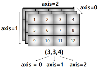

mathmatical functions

np.something 으로 호출

exponential
exp, expml, exp2, log, log10, log1p, log2, power, sqrt
trigonometric
sin, cos, tan, acsin, arccos, atctan
hyperbolic
sinh, cosh, tanh, acsinh, arccosh, atctanh

vstack & hstack

numpy array를 합치는(붙이는) 함수

a = np.array([1, 2, 3])
b = np.array([2, 3, 4])
np.vstack((a, b))
# array([[1, 2, 3],
#        [2, 3, 4]])

a = np.array([[1], [2], [3]])
b = np.array([[2], [3], [4]])
np.hstack((a, b))
# array([[1, 2],
#        [2, 3],
#        [3, 4]])

concatenate

numpy array를 합치는(붙이는) 함수

a = np.array([[1, 2, 3]])
b = np.array([[2, 3, 4]])
np.concatenate((a, b), axis = 0)
# array([[1, 2, 3],
#        [2, 3, 4]])

a = np.array([[1, 2], [3, 4]])
b = np.array([[5, 6]])
np.concatenate((a, b.T), axis= 1)
# array([[1, 2, 5],
#        [3, 4, 6]])

array operations

numpy는 array 간의 기본적인 사칙 연산을 지원한다.

test_a = np.array([[1, 2, 3], [4, 5, 6]], float)
test_a + test_a # Matrix + Matrix 연산
# array([[ 2.,  4.,  6.],
#        [ 8., 10., 12.]])

test_a - test_a # Matrix + Matrix 연산
# array([[0., 0., 0.],
#        [0., 0., 0.]])

test_a * test_a  # Matrix 내 element 들 간 같은 위치에 있는 값들끼리 연산
# array([[ 1.,  4.,  9.],
#        [16., 25., 36.]])

dot product

Matrix의 기본 연산, dot 함수를 사용한다.

test_a = np.arange(1, 7).reshape(2, 3)
test_b = np.arange(7, 13).reshape(3, 2)
test_a.dot(test_b)
# array([[ 58,  64],
#        [139, 154]])

transpose

transpose 또는 T attribute 사용

test_a = np.arange(1, 7).reshape(2, 3)
# array([[1, 2, 3],
#        [4, 5, 6]])

test_a.transpose()
# array([[1, 4],
#        [2, 5],
#        [3, 6]])

test_a.T
# array([[1, 4],
#        [2, 5],
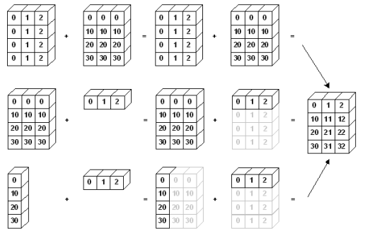
#        [3, 6]])

broadcasting

Shape이 다른 배열 간 연산을 지원하는 기능

test_matrix = np.array([[1, 2, 3,], [4, 5, 6]], float)
scalar = 3

test_matrix + scalar # Matrix - Scalar 덧셈
# array([[4., 5., 6.],
#        [7., 8., 9.]])

test_matrix - scalar # Matrix - Scalar 뺄셈
test_matrix * scalar # Matrix - Scalar 곱셈
test_matrix / scalar # Matrix - Scalar 나눗셈
test_matrix // scalar # Matrix - Scalar 몫
test_matrix ** scalar # Matrix - Scalar 제곱

Scalar - vector 외에도 vector - matrix 간의 연산도 지원

test_matrix = np.arange(1, 13).reshape(4, 3)
test_vector = np.arange(10, 40, 10)
test_matrix + test_vector
# array([[11, 22, 33],
#        [14, 25, 36],
#        [17, 28, 39],
#        [20, 31, 42]])

numpy performance

일반적으로 속도는 for loop < list comprehension < numpy 순이다.
100,000,000 번의 loop를 돌 때, 약 4배 이상의 성능 차이를 보인다.
numpy는 c로 구현되어 있어, 성능을 확보하지만 파이썬의 장점인 dynamic typing을 포기한다.
대용량 계산에서 사용된다.
concatenate처럼 계산이 아닌, 할당에서는 연산 속도의 이점이 없다.

def sclar_vector_product(scalar, vector):
    result = []
    for value in vector:
        result.append(scalar * value)
    return result
    
iternation_max = 100000000

vector = list(range(iternation_max))
scalar = 2

%timeit sclar_vector_product(scalar, vector) # for loop을 이용한 성능
%timeit [scalar * value for value in range(iternation_max)]
# list comprehension을 이용한 성능
%timeit np.arange(iternation_max) * scalar # numpy를 이용한 성능

comparisons

all & any

array의 데이터 전부(and) 또는 일부(or)가 조건에 만족하는지 여부를 반환

any 하나라도 조건에 만족한다면 true
all 모두가 조건에 만족한다면 True

a = np.arange(10)
a
# array([0, 1, 2, 3, 4, 5, 6, 7, 8, 9])

np.any(a > 5), np.any(a < 0)
# (True, False)

np.all(a > 5), np.all(a < 10)
# (False, True)

comparison operation

numpy 는 배열의 크기가 동일할 때 element간 비교의 결과를 boolean type으로 반환

test_a = np.array([1, 3, 0], float)
test_b = np.array([5, 2, 1], float)
test_a > test_b
# array([False,  True, False])

test_a == test_b
# array([False, False, False])

(test_a > test_b).any()
# True

a = np.array([1, 3, 0], float)
np.logical_and(a > 0, a < 3) # and 조건의 condition
# array([ True, False, False])

b = np.array([True, False, True], bool)
np.logical_not(b)
# array([False,  True, False])

c = np.array([False, True, False], bool)
np.logical_or(b, c)
# array([ True,  True,  True])

np.where

a = np.array([1, 3, 0], float)
np.where(a > 0, 3, 2) # where(condition, True, False)
# array([3, 3, 2])

a = np.arange(10)
np.where(a > 5) # Index 값 반환
# (array([6, 7, 8, 9], dtype=int64),)

a = np.array([1, np.NaN, np.Inf], float)
np.isnan(a) # Not a Number
# array([False,  True, False])

np.isfinite(a) # is finite number
# array([ True, False, False])

argmax & argmin

array내 최대값 또는 최속밧의 index를 반환

a = np.array([1, 2, 4, 5, 8, 78, 23, 3])
np.argmax(a), np.argmin(a)
# (5, 0)

axis 기반의 반환

a = np.array([[1, 2, 4, 7], [9, 88, 6, 45], [9, 76, 3, 4]])
a
# array([[ 1,  2,  4,  7],
#       [ 9, 88,  6, 45],
#       [ 9, 76,  3,  4]])

np.argmax(a, axis = 1), np.argmin(a, axis = 0)
# (array([3, 1, 1], dtype=int64), array([0, 0, 2, 2], dtype=int64))

boolean & fancy index

boolean index

특정 조건에 따른 값을 배열 형태로 추출

comparison operation 함수들도 모두 사용 가능하다.

test_array = np.array([1, 4, 0, 2, 3, 8, 9, 7], float)
test_array > 3
# array([False,  True, False, False, False,  True,  True,  True])

test_array[test_array > 3] # 조건이 True인 index의 element만 추출
# array([4., 8., 9., 7.])

condition = test_array < 3
test_array[condition]
# array([1., 0., 2.])

fancy index

numpy는 array를 index value로 사용해서 값 추출

a = np.array([2, 4, 6, 8], float)
b = np.array([0, 0, 1, 3, 2, 1], int) # 반드시 integer로 선언
a[b] # bracket index, b 배열의 값을 index로 하여 a의 값들을 추출함
array([2., 2., 4., 8., 6., 4.])

a.take(b) # take함수: bracket index와 같은 효과
# array([2., 2., 4., 8., 6., 4.])

matrix 형태의 데이터도 가능하다.

a = np.array([[1, 4,], [9, 16]], float)
b = np.array([0, 0, 1, 1, 0], int)
c = np.array([0, 1, 1, 1, 1], int)
a[b, c] # b를 row index, c를 column index로 변환하여 표시함
# array([ 1.,  4., 16., 16.,  4.])

numpy data I/O

loadtxt & savetxt

text type의 데이터를 읽고 저장하는 기능

a = np.loadtxt('./populations.txt')

a_int = a.astype(int) # int type 변환

np.savetxt('int_dat.csv', a_int, fmt = '%.2e' delimiter = ',', ) # int_data.csv로 저장

numpy object (npy)

np.save('npy_test', arr = a_int)

a_test = np.load(file = 'npy_test.npy')
a_test

Mathematics for Artificial Intelligence

Vector

벡터는 숫자를 원소로 가지는 리스트(list) 또는 배열(array) 입니다.

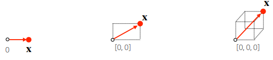
벡터는 공간에서 한 점을 나타냅니다.
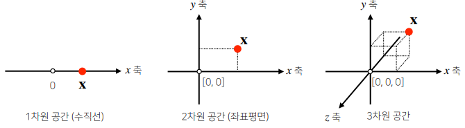
벡터는 원점으로부터 상대적 위치를 표현합니다.

x = [1, 7, 2]
x = np.array([1, 7, 2])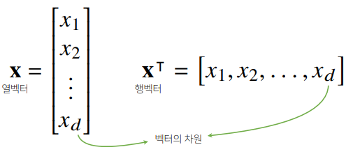

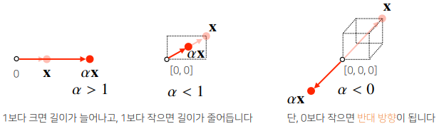
벡터에 숫자를 곱해주면 길이만 변합니다.
벡터끼리 같은 모양을 가지면 덧셈, 뺄셈, 성분곱을 계산할 수 있습니다.

x = np.array([1, 7, 2])
y = np.array([5, 2, 1])
x + y
# array([6, 9, 3])

x - y
# array([-4,  5,  1])

x * y
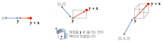
# array([ 5, 14,  2])

벡터의 덧셈

두 벡터의 덧셈은 다른 벡터로부터 상대적 위치이동을 표현합니다.

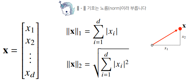
벡터의 노름

벡터의 노름(norm)은 원점에서부터의 거리를 말합니다.

L1 노름은 각 성분의 변화량의 절대값을 모두 더합니다.
L2 노름은 피타고라스 정리를 이용해 유클리드 거리를 계산합니다.

def l1_norm(x):
    x_norm = np.abs(x)
    x_norm = np.sum(x_norm)
    return x_norm

def l2_norm(x):
    x_norm = x * x
    x_norm = np.sum(x_norm)
    x_norm = np.sqrt(x_norm)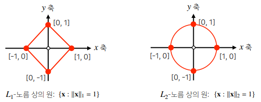
    return x_norm

노름을 쓰는 이유
노름의 종류에 따라 기하학적 성질이 달라집니다.
- 머신러닝에선 각 성질들이 필요할 때가 있으므로 둘 다 사용합니다.
  원: 원점에서부터의 거리 (L1, L2 노름이 다르다)

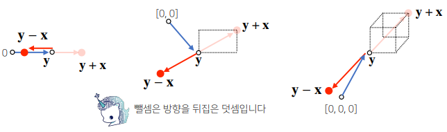
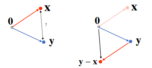
두 벡터 사이의 거리

L1, L2 노름을 이용해 두 벡터 사이의 거리를 계산할 수 있습니다.
벡터 사이의 거리를 계산할 때는 벡터의 뺄셈을 이용합니다.
||y - x|| = ||x - y|| (뺄셈을 거꾸로 해도 거리는 같습니다.)

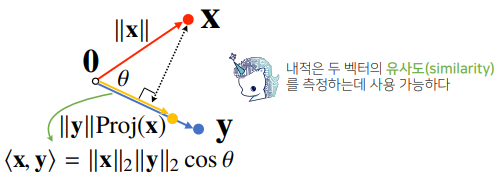
두 벡터 사이의 각도

제2 코사인 법칙에 의해 두 벡터 사이의 각도를 계산할 수 있다. (n차원에서도 가능하다.)
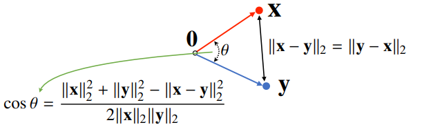
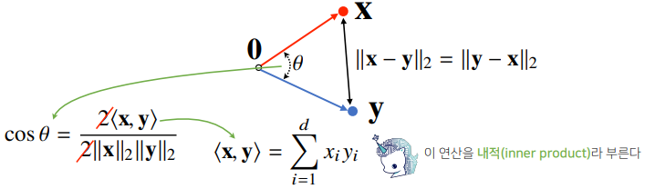
분자를 쉽게 계산하는 방법이 내적이다.
L2 노름에서만 가능하다.

def angle(x, y):
    v = np.inner(x, y) / (l2_norm(x) * l2_norm(y))
    theta = np.arccos(v)
    return theta

내적은 정사영(orthogonalprojection)된 벡터의 길이와 관련 있다.

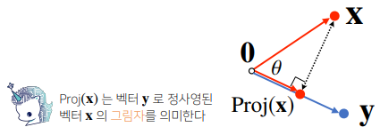
Proj(x)의 길이는 코사인법칙에 의해 || x || cosθ가 된다.

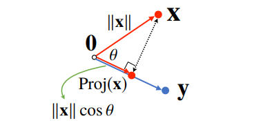
내적은 정사영의 길이를 벡터의 길이만큼 조정한 값이다.

Matrix 행렬

행렬(matrix)은 벡터를 원소로 가지는 2차원 배열입니다.

numpy에선 행(row)이 기본 단위이다. (numpy -> 행 벡터로 표현)

X = np.array([[1, -2, 3], 
              [7, 5, 0], 
              [-2, -1, 2]])

행렬은 행(row)과 열(column)이라는 인덱스(index)를 가집니다.
행렬의 특정행(열)을 고정하면 행(열)벡터라 부릅니다.

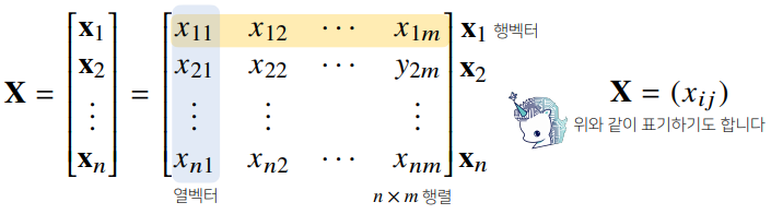
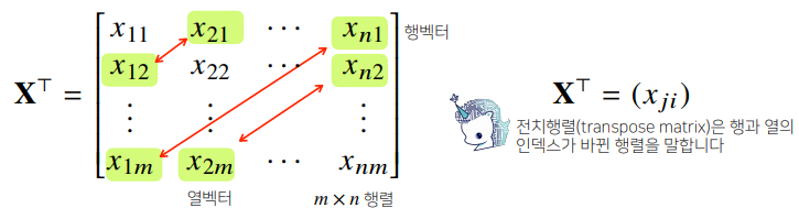
전치행렬(transpose matrix)은 행과 열의 인덱스가 바꾸니 행렬을 말합니다.

행렬의 이해

벡터가 공간에서 한 점을 의미한다면 행렬은 여러 점들을 나타냅니다.
행렬의 행벡터 xi는 i번째 데이터를 의미합니다.

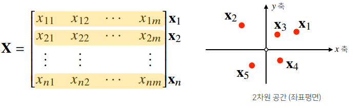
행렬의 xij는 i번째 데이터의 j번째 변수의 값을 말합니다.

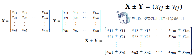
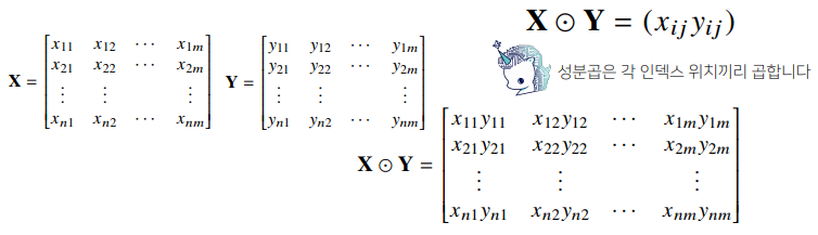
행렬끼리 같은 모양을 가지면 덧셈, 뺄셈, 성분곱을 계산할 수 있습니다.

스칼라 곱도 벡터와 차이가 없습니다.

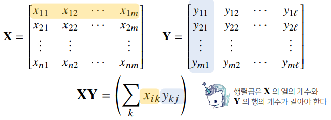
행렬 곱셈

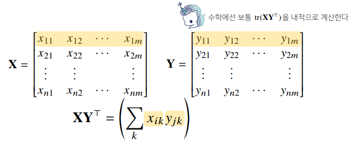
행렬곱셈(matrixmultiplication)은 i번째 행벡터와 j번째 열벡터사이의 내적을성분으로 가지는 행렬을 계산합니다.

X = np.array([[1, -2, 3],
              [7, 5, 0],
              [-2, -1, 2]])
              
Y = np.array([[0, 1],
              [1, -1],
              [-2, 1]])
X @ Y
# array([[-8,  6],
#        [ 5,  2],
#        [-5,  1]])

행렬 내적

넘파이의 np.inner는 i번째 행벡터와 j번째 행벡터 사이의 내적을 성분으로 가지는 행렬을 계산합니다.

수학에서 말하는 내적과는 다르므로 주의합니다.

X = np.array([[1, -2, 3],
              [7, 5, 0],
              [-2, -1, 2]])
              
Y = np.array([[0, 1, -1],
              [1, -1, 0]])

np.inner(X, Y)
# array([[-5,  3],
#        [ 5,  2],
#        [-3, -1]])

행렬의 이해

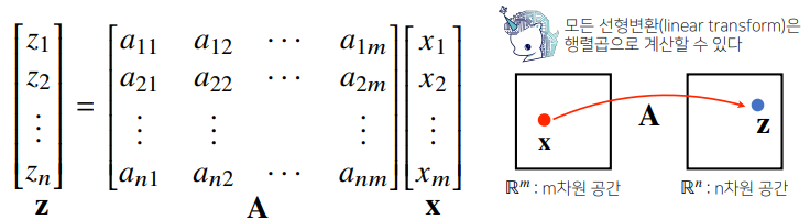
행렬은 벡터공간에서 사용되는 연산자(operator)로 이해한다.

행렬곱을 통해 벡터를 다른 차원의 공간으로 보낼 수 있습니다.
행렬곱을 통해 패턴을 추출할 수 있고 데이터를 압축할 수도 있습니다.

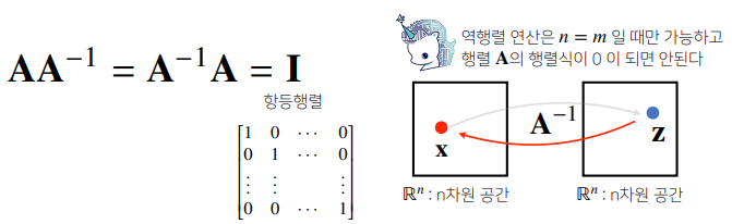
역행렬

어떤 행렬 A의 연산을 거꾸로 되돌리는 행렬을 역행렬(inversematrix)이라 부른다.

역행렬은 행과 열의 숫자가 같고 행렬식(determinant)이 0이 아닌 경우에만 계산할 수 있다.

X = np.array([[1, -2, 3],
              [7, 5, 0],
              [-2, -1, 2]])

np.linalg.inv(X)
# array([[ 0.21276596,  0.0212766 , -0.31914894],
#        [-0.29787234,  0.17021277,  0.44680851],
#        [ 0.06382979,  0.10638298,  0.40425532]])

X @ np.linalg.inv(X)
# array([[ 1.00000000e+00, -1.38777878e-17,  0.00000000e+00],
#        [ 0.00000000e+00,  1.00000000e+00,  0.00000000e+00],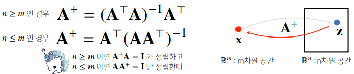
#        [-2.77555756e-17,  0.00000000e+00,  1.00000000e+00]])

만일 역행렬을 계산할 수 없다면 유사역행렬(pseudo-inverse) 또는 무어펜로즈(Moore-Penrose)역행렬을 이용한다.

Y = np.array([[0, 1],
              [1, -1],
              [-2, 1]])
              
np.linalg.pinv(Y)
# array([[ 5.00000000e-01,  1.11022302e-16, -5.00000000e-01],
#        [ 8.33333333e-01, -3.33333333e-01, -1.66666667e-01]])

np.linalg.pinv(Y) @ Y
# array([[ 1.00000000e+00, -2.22044605e-16],
#        [ 1.11022302e-16,  1.00000000e+00]])

np.linalg.pinv를 이용하면 연립방정식의 해를 구할 수 있다.
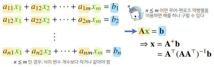
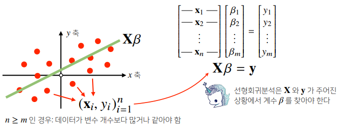
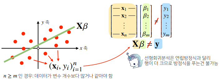
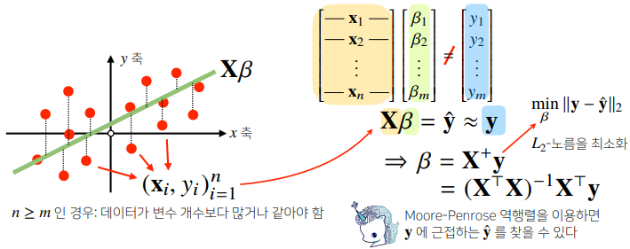
np.linalg.pinv를 이용하면 데이터를 선형모델(linearmodel)로 해석하는 선형회귀식을 찾을 수 있다.

# Scikit Learn 을 활용한 회귀분석
from sklearn.linear_model import LinearRegression
model = LinearRegression()
model.fit(X, y)
y_test = model.predict(x_test)

# Moore-Penrose 역행렬 (같은 방법이지만 결과가 다르다.)
beta = np.linalg.pinv(X) @ y
y_test = np.append(x_test) @ beta 

# Moore-Penrose 역행렬
X_ = np.array([np.append(x, [1]) for x in X) # intercept 항 추가
beta = np.linalg.pinv(X) @ y
y_test = np.append(x_test) @ beta

Lee

초보 개발자입니다

이전 포스트

Ai tech Day5

다음 포스트

Ai tech Day6

Numerical Python (numpy)

numpy

ndarray

Handling shape

reshape

flatten

indexing & slicing

indexing

slicing

creation function

arange

zeros

ones

empty

something_like

identity

eye

diag

random sampling

operation functions

sum

mean & std

axis

mathmatical functions

vstack & hstack

concatenate

array operations

dot product

transpose

broadcasting

numpy performance

comparisons

all & any

comparison operation

np.where

argmax & argmin

boolean & fancy index

boolean index

fancy index

numpy data I/O

loadtxt & savetxt

numpy object (npy)

Mathematics for Artificial Intelligence

Vector

벡터의 덧셈

벡터의 노름

두 벡터 사이의 거리

두 벡터 사이의 각도

Matrix 행렬

행렬의 이해

행렬 곱셈

행렬 내적

행렬의 이해

역행렬

Ai tech Day5

Ai tech Day7

0개의 댓글