Hyperparameter Tuning 효율적으로 하기
Intro.
- 가장 기본적인 방법으로 grid vs random 있다.
- 최근에는 베이지안 기반 기법들이 주도하고 있다.
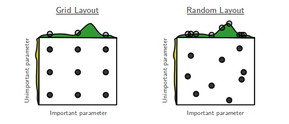
Grid Layout
learning rate 0.1, 0.01, 0.001 → ...
batchsize 32, 64, 128 → ...
조합들을 적용해가며 가장 좋은 하이퍼파라미터를 찾는다.
Random Layout
말 그대로 랜덤으로 적용해본다.
Ray
![]()
특징
- multi-node multi processing 지원하는 모듈이다.
- ML/DL의 병렬 처리를 위해 개발된 모듈이다.
- 기본적으로 현재의 분산병렬 ML/DL 모듈의 표준
- Hyperparameter Search를 위한 다양한 모듈을 제공한다.
Code
data_dir = os.path.abspath("./data")
load_data(data_dir)

# search space 지정
config = {
    "l1": tune.sample_from(lambda _: 2 ** np.random.randint(2, 9)),
    "l2": tune.sample_from(lambda _: 2 ** np.random.randint(2, 9)),
    "lr": tune.loguniform(1e-4, 1e-1),
    "batch_size": tune.choice([2, 4, 8, 16])
}

# 학습 스케줄링 알고리즘 지정
scheduler = ASHAScheduler( # 가망이 없는 것들 제외하는 알고리즘
    metric="loss",
    mode="min",
    max_t=max_num_epochs,
    grace_period=1,
    reduction_factor=2)

# 결과 출력 양식 지정
reporter = CLIReporter( # command line 출력
    # parameter_columns=["l1", "l2", "lr", "batch_size"],
    metric_columns=["loss", "accuracy", "training_iteration"])

# 병렬처리양식으로 실행
result = tune.run(
    partial(train_cifar, data_dir=data_dir),# 데이터 쪼개기
		# 한번 trial시 사용하는 cpu,gpu
    resources_per_trial={"cpu": 2, "gpu": gpus_per_trial},
    config=config,
    num_samples=num_samples,
    scheduler=scheduler,
    progress_reporter=reporter)

# 가장 좋은 결과 가져오기
best_trial = result.get_best_trial("loss", "min", "last")
print("Best trial config: {}".format(best_trial.config))
print("Best trial final validation loss: {}".format(
    best_trial.last_result["loss"]))
print("Best trial final validation accuracy: {}".format(
    best_trial.last_result["accuracy"]))

best_trained_model = Net(best_trial.config["l1"], best_trial.config["l2"])
하지만 하이퍼파라미터 튜닝보다 좋은 데이터가 더 중요하다는 점 잊지말자!

나는야 호기심 많은 느림보🤖
HPO 에서 Random Search와 Grid Search의 차이점은 인터뷰에서 자주 나오는 문제이기 때문에 어떤 차이점이 있는지 자세하게 알아두면 좋습니다.