팔당댐 수위 예측 AI 대회 코드 #3 EDA실행

1. 외부 데이터 합치기

df = pd.merge(rf_df, water_df, on="timestamp")
df = df.drop(["ymdhm_x", "ymdhm_y"], axis=1)

대회측에서 제공해준 강수량 데이터와 물 데이터를 먼저 합쳐준다
(rf_df와 water_df는 2-1에서 수정해둔 그 상태 그대로 이용)

external = pd.read_csv("./gimpo_seoul_namyang.csv")
external.rename(columns={"time": "timestamp"}, inplace=True)
external[external.columns[1:]] = external[external.columns[1:]].applymap(lambda x : x * 100)
df = pd.merge(df, external[["timestamp", "wl_1019675", "wl_1018640", "wl_1018610"]], on="timestamp")
df.head()

1편에서 가공해둔 외부 데이터 (gimpo_seoul_namyang.csv)를 불러내여 df에 합쳐준다.

다음과 같이 끝에 wl_1019675 (전류리 수위 데이터)가 추가됐음을 확인할 수 있다.

​

그러던 중 한강의 수위가 서해의 조수간만의 차, 조위에 영향을 많이 받는 다는 것을 알게되었다.

(한강에 관한 논문을 살면서 처음 읽어보았다..)

출처

경인항의 조위를 2013년부터 2022년까지 1분 단위로 수집하였고, 이를 10분 단위로 가공하여 활용하였다.
(최종 제출에서는 서해와 가장 가까운 행주대교의 수위를 예측하는 모델에만 활용하였다)

​

수위 데이터와 마찬가지로 예측하는 일시의 10분 전까지만 훈련에 활용하였다
(Data Leakage 아님!)

tide = pd.read_csv("tide_data_done.csv")
tide["timestamp"] = tide["time"].apply(str_to_unixtime)
df = pd.merge(df, tide[["timestamp", "tide"]], on="timestamp")

조위 데이터 역시 df에 추가해준다.

sample_submission["timestamp"] = sample_submission["ymdhm"].apply(str_to_unixtime)

df.index = pd.to_datetime(df.timestamp, unit="s")
df.sort_index(inplace=True)
df.tail()

꼬리를 찍어보면

주어진 데이터에는 다음과 같이 2022년 6월~7월18일 까지의 수위데이터가 0으로 비워져 있는 것을 알 수 있다.

(662:청담대교, 680:잠수교, 683:한강대교, 630:행주대교)

2. 정답 데이터 추가

​

1에서 외부데이터를 이용하여 미리 확보해둔 솔루션파일(2022년 6월~7월18일 까지의 수위데이터)을 불러온다.

solution = pd.read_csv("solution.csv")

solution.index = pd.to_datetime(solution.timestamp, unit="s")
solution.sort_index(inplace=True)

index를 다시 datetime으로 바꿔준 다음 정렬해준다.
그러면 솔루션 파일은

다음과 같이 datetime을 기준으로 정렬된다.

temp_test_df = df.loc[solution.index]
for col in solution.columns[1:]:
    temp_test_df[col] = solution[col]

그 다음 df의 0으로 채워져있던 2022년 6월~7월18일 까지의 수위데이터 행에
정답데이터를 넣어준다.

df = pd.concat([df.iloc[:-len(sample_submission), :], temp_test_df], axis=0)

정답데이터가 추가된 2022년 데이터까지 합쳐서 df를 최종적으로 만들어준다.

3. 학습을 위한 10분전 데이터로 만들기

이번 대회는 10분 뒤의 한강의 수위를 예측하는 대회이다 보니, 현재를 기준으로 10분 전의 데이터는 전부 사용해도 된다.

따라서 10분을 당긴 데이터를 하나 만들어준다

(662:청담대교, 680:잠수교, 683:한강대교, 630:행주대교)

target_columns = ["wl_1018662", "wl_1018680", "wl_1018683", "wl_1019630"]
target = df[target_columns]
target = target.shift(-1)
target.tail()

shift가 잘 된 것을 확인할 수 있다.

train_df = df.iloc[:-len(sample_submission) - 1, :]
test_df = df.iloc[-len(sample_submission) - 1:-1, :]
target = target.iloc[:-1]

10분전 데이터를 이용하기 위한 train set과 test set을 만들어주고 target 데이터도 7/18일 23시 50분 값을 잘라준다.

4. 결측값 처리

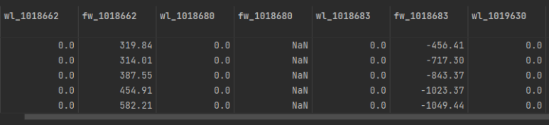
nan_cols = [col for col in train_df.columns if train_df[col].isnull().any()]
for col in nan_cols:
    print(col, train_df[col].isnull().sum())

결측값을 찍어보면 다음과 같다

유독 잠수교의 유량데이터(fw_1018680)에만 결측값이 높은 것을 확인할 수 있다.

y_train_full = target.iloc[:len(train_df)]
X_train_full = train_df.copy()
X_test = test_df.copy()

앞서 10분전으로 shift해둔 target (정답포함)을 train_df의 길이만큼 잘라주어 y_train_full로 만들어준다.
이후 x_train과 test를 모두 만들어준다. ( 모든 데이터가 전부 포함되었기 때문에 full을 붙여주었다)

X_train_full = X_train_full.drop(["fw_1018680"], axis=1)
X_test = X_test.drop(["fw_1018680"], axis=1)

잠수교의 유량 데이터는 nan값이 너무 많으므로 그냥 버려준다.

​

남은 결측값들은 quadratic interpolation으로 채워준다.

interpolation_method = "quadratic"
imputed_X_train = X_train_full.interpolate(method=interpolation_method, axis=0)
imputed_X_test = X_test.interpolate(method=interpolation_method, axis=0)
imputed_y_train = y_train_full.interpolate(method=interpolation_method, axis=0)

print(imputed_X_train.isna().sum().sum())
print(imputed_X_test.isna().sum().sum())
print(imputed_y_train.isna().sum().sum())

확인해보면 결측치가 말끔하게 지워진 것을 확인할 수 있다.

5. 시간 데이터를 24시간 기준으로 추가 feature 생성

imputed_X_train["hour"] = imputed_X_train.index.hour
imputed_X_test["hour"] = imputed_X_test.index.hour

6. 시간에 따른 추가 feature 생성

기본적으로 모든 feature는 예측하고자 하는 다리의 10분 전의 데이터들을 활용해야한다

• 현재의 데이터들로 미래의 한강 수위를 예측하는 모델을 만들어야하기 때문

함수명은 day_shift로 했지만 사실 10분씩 shift해주는 함수이다
(정식 명칭은 10_min_shift 정도로 하면 되겠다)

from pandas.tseries.offsets import DateOffset

def day_shift(df, day_shift=None, cols=None):
    shift_df = df.copy()
    shift_list = [i for i in range(1,300) if imputed_X_train["wl_1018662"].autocorr(i) > 0.88]
    if day_shift is None:
        for col in df.columns:
            for i in shift_list:
                shift_df["{}_{}min_prev".format(col, i * 10)] = df[col].shift(i, freq=DateOffset(minutes=10))
    else:
        if cols is None:
            for col in df.columns:
                for i in range(1, day_shift + 1):
                    shift_df["{}_{}min_prev".format(col, i * 10)] = df[col].shift(i, freq=DateOffset(minutes=10))
        else:
            for col in cols:
                for i in range(1, day_shift + 1):
                    shift_df["{}_{}min_prev".format(col, i * 10)] = df[col].shift(i, freq=DateOffset(minutes=10))
    return shift_df

day_shift, cols에 따라 원하는 만큼, 원하는 행을 골라서 shift 할 수 있는 함수이다.

각 종속 변수를 auto correlation를 찍어보았다
(유능한 github copilot 가 있으니 찍는 코드는 따로 기록하지 않도록 하겠다)

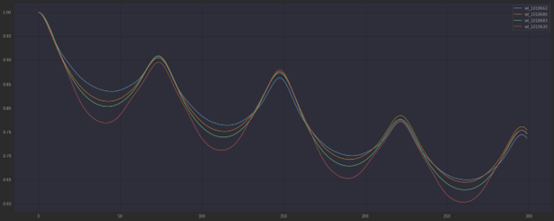
그래프를 통한 분석 결과 170분 전까지가 가장 상관관계가 높음을 알 수 있다.

따라서 우리는 데이터에 170분 전까지의 데이터를 feature로 추가로 사용하기로 결정했다.

shift_day = 17

DateOffset을 10분으로 설정해두었기 때문에
shift_day를 17로 설정하면 170분 전까지의 데이터를 사용할 수 있다.

full_df = pd.concat([imputed_X_train, imputed_X_test], axis=0)
shifted_full = day_shift(full_df, shift_day)

결측값을 채워넣은 imputed 데이터들을 합쳐 full_df를 만들어주고
170분 전까지의 데이터를 feature로 추가한 shifted_full 데이터를 만들어주었다.

shifted_X_train = shifted_full.iloc[:len(imputed_X_train), :]
shifted_X_test = shifted_full.iloc[len(imputed_X_train):, :]
shifted_X_train = shifted_X_train.iloc[shift_day:, :]

shiftedfull 데이터에서 다시 train 데이터 셋과 test 데이터 셋을 나누어준다
day_shift를 해주면 '170분전 prev' 행은 17개의 nan 값이 존재하므로 잘라준다

try:
    imputed_y_train = imputed_y_train.values
except:
    pass

pandas에서 numpy로 바꿔준다

shifted_y_train = imputed_y_train[shift_day:, :]

X train에서도 17개 잘라줬으니 y train에서도 똑같이 잘라준다

try:
    shifted_y_train = shifted_y_train.values
except:
    pass

같은 작업을 똑같이 진행해준다

# calculate root mean squared error between test_pred and solution on each columns
def rmse(y_true, y_pred):
    return np.sqrt(np.mean((y_true - y_pred) ** 2))

rmse를 정의해준다.
솔루션을 이미 확보하였기 때문에 submission파일을 제출해보지 않아도 우리의 성적을
자체적으로 찍어볼 수 있다.

7. moving average

시간에 따른 각 값의 변화량을 대략적으로 알기 위해 moving average를 추가하였다.

행주대교, 강화대교, 한강대교, 잠수교, 팔당대교, 광진교, 청담대교 7개의 다리의 수위를 moving average하여

새 feature로 만들어주었다.

for window in range(5,30,5):
    cols = ["wl_1018662", "wl_1018680", "wl_1018683", "wl_1019630", "wl_1018610", "wl_1018640", "tide_level"]
    for col in cols:
        shifted_X_train["{}_{}_ma".format(window, col)] = shifted_X_train[col].rolling(window=window).mean()
        shifted_X_test["{}_{}_ma".format(window, col)] = shifted_X_test[col].rolling(window=window).mean()

각각 5, 10, 15, 20, 25의 window 크기로 averaging 했다. 즉 총 35개의 새 feature를 추가했다.

​