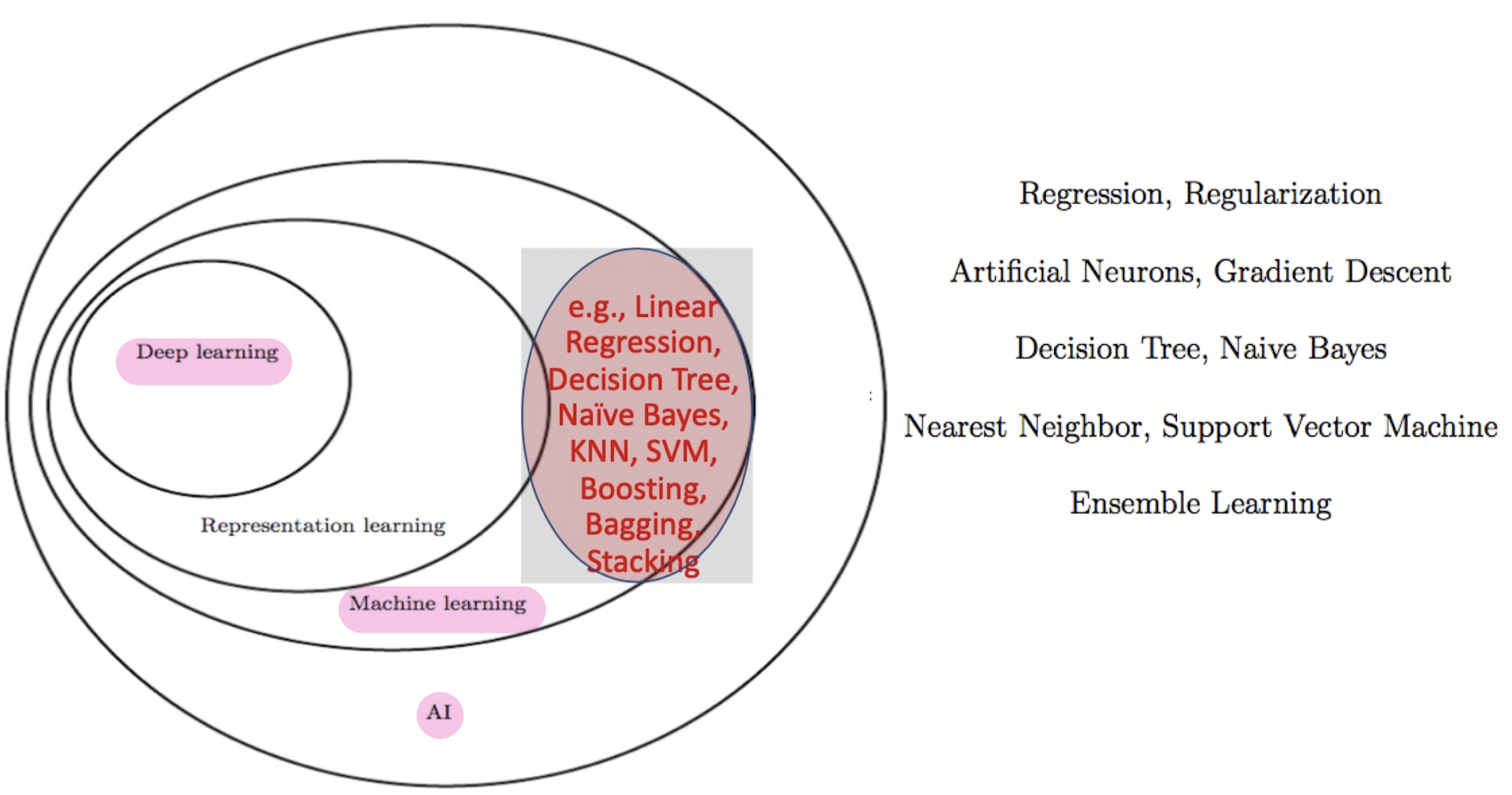
1. machine learning
How does a machine learning learns?
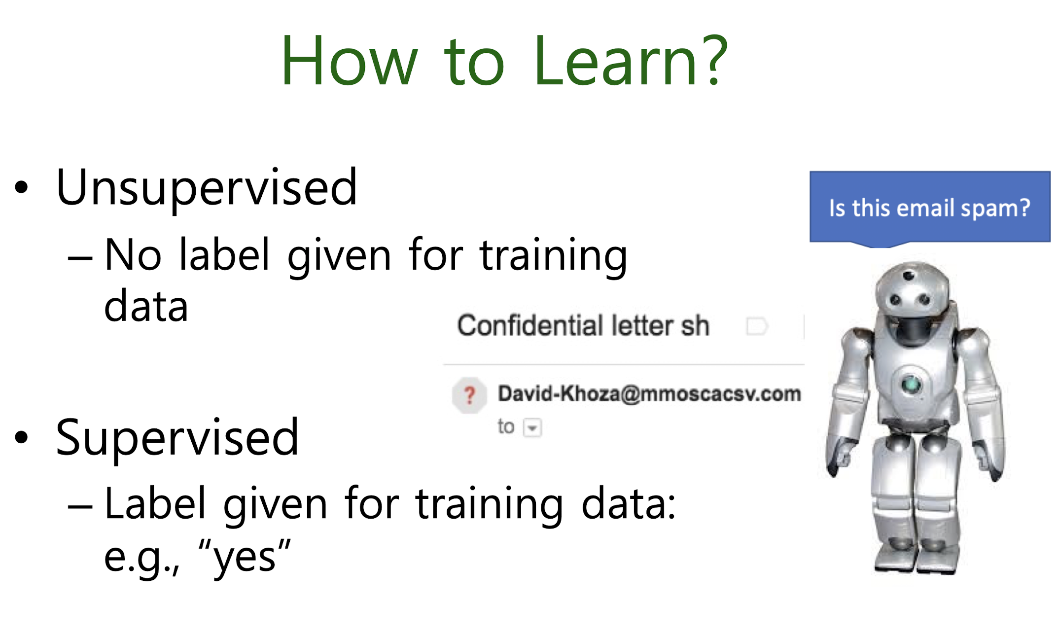
Unsupervised

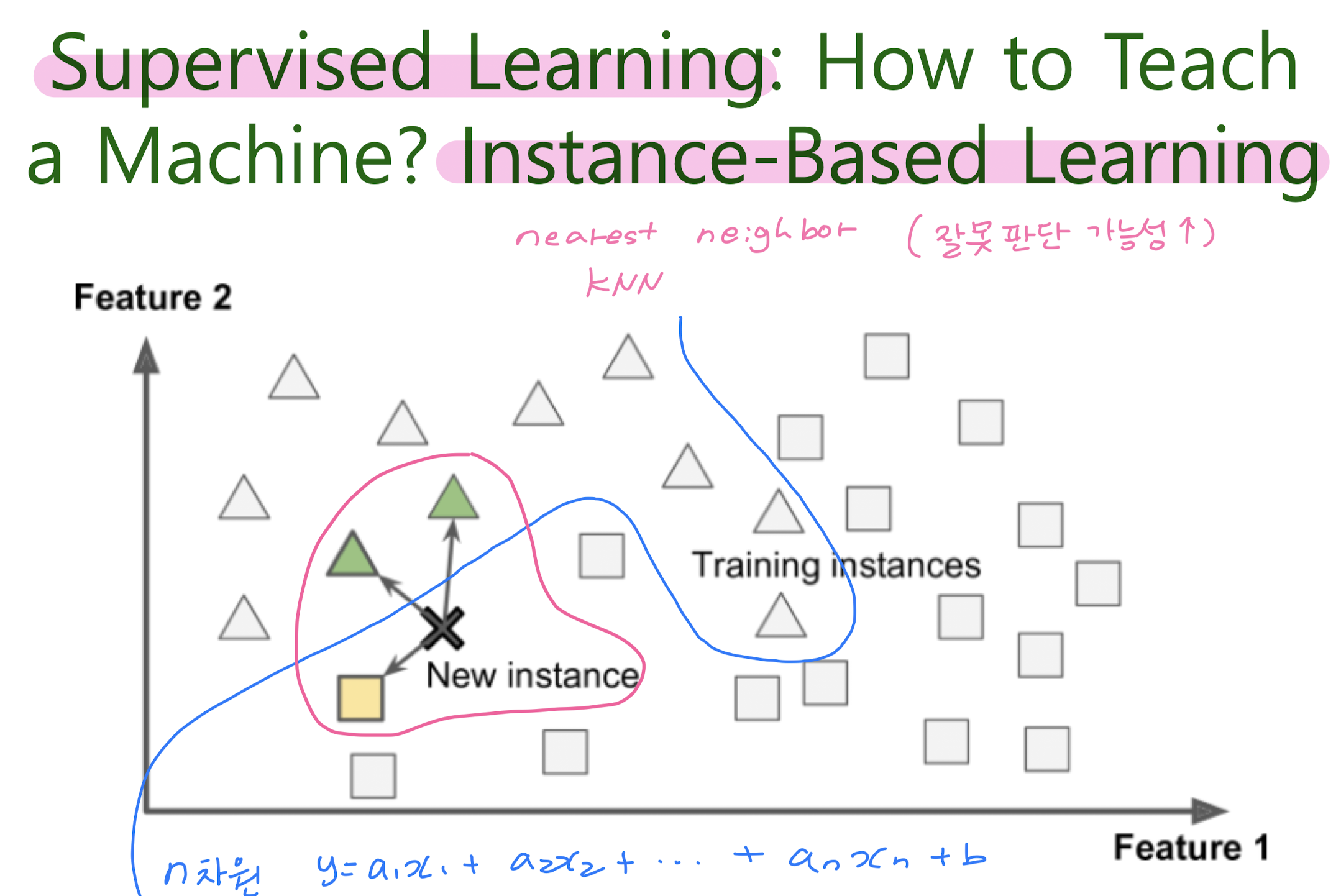
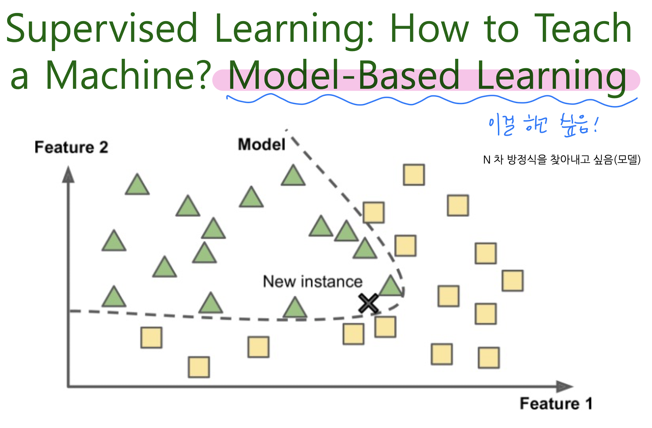
Supervised
instance-based learning / model-based learning
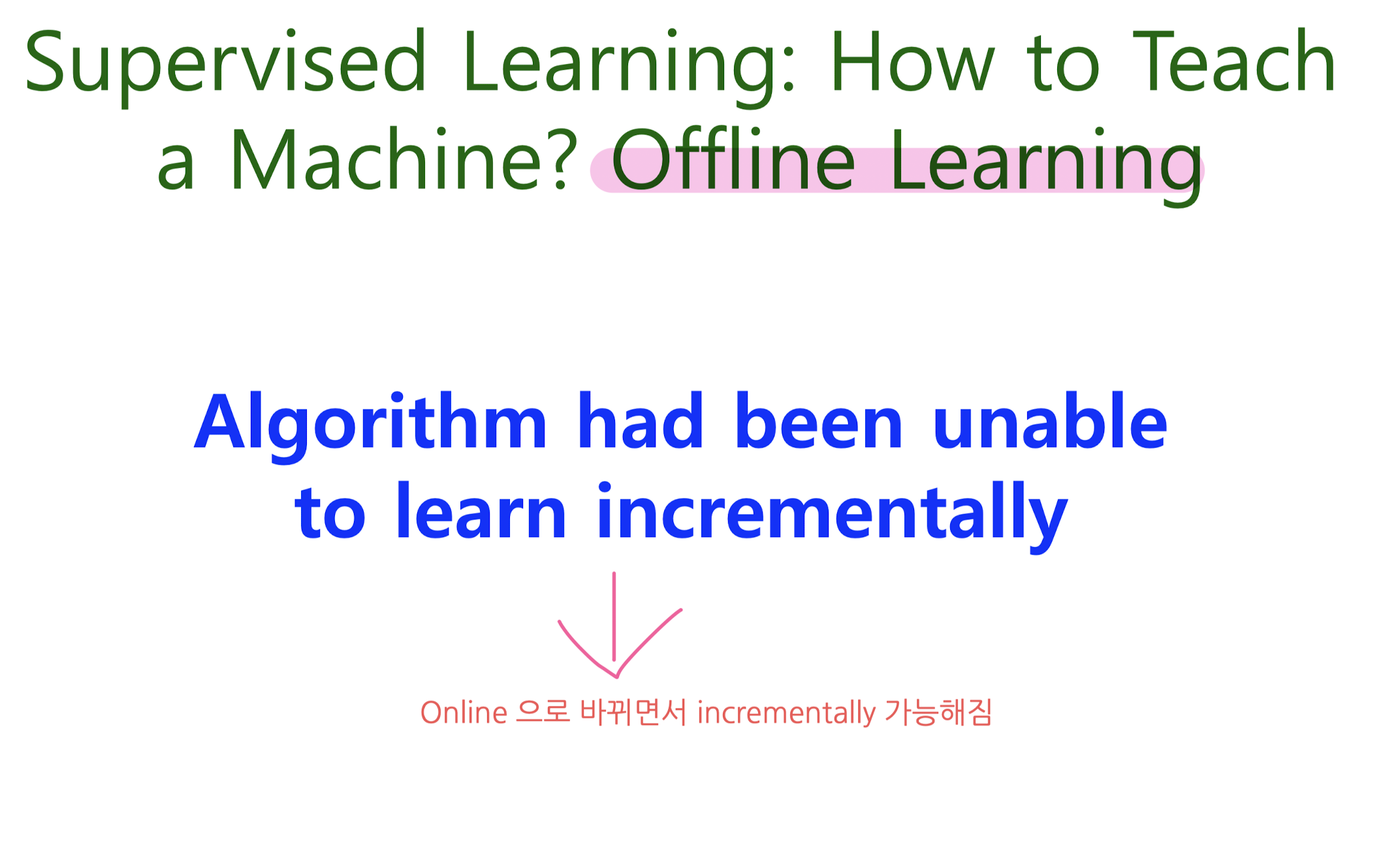
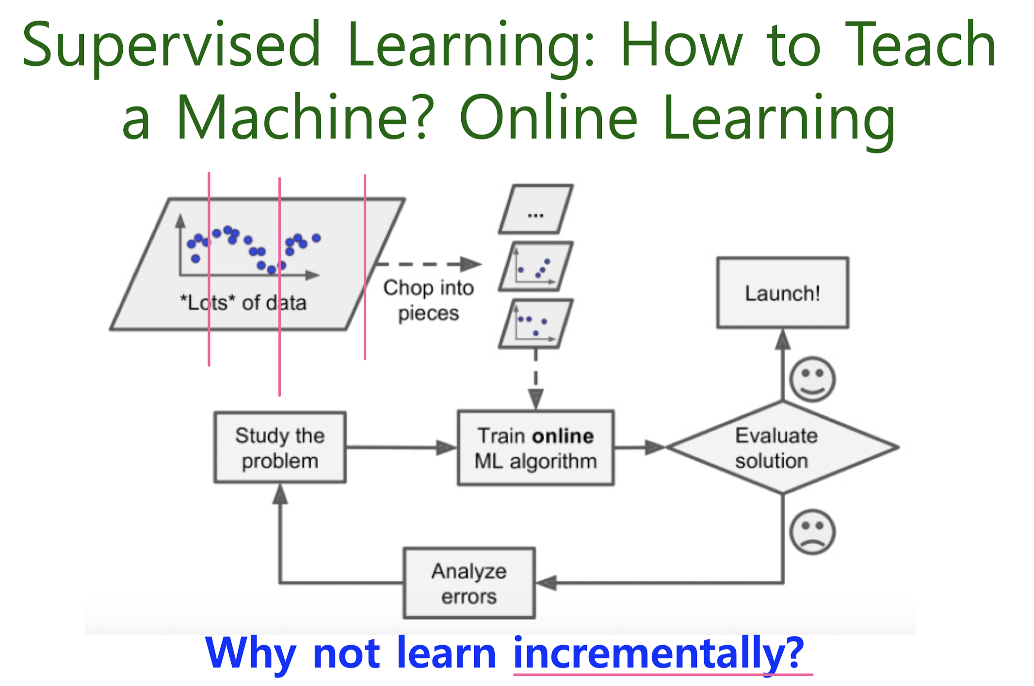
Offline learning / Online learning
Algorithm scope
2. Mathematics for ML
Linear Algebra
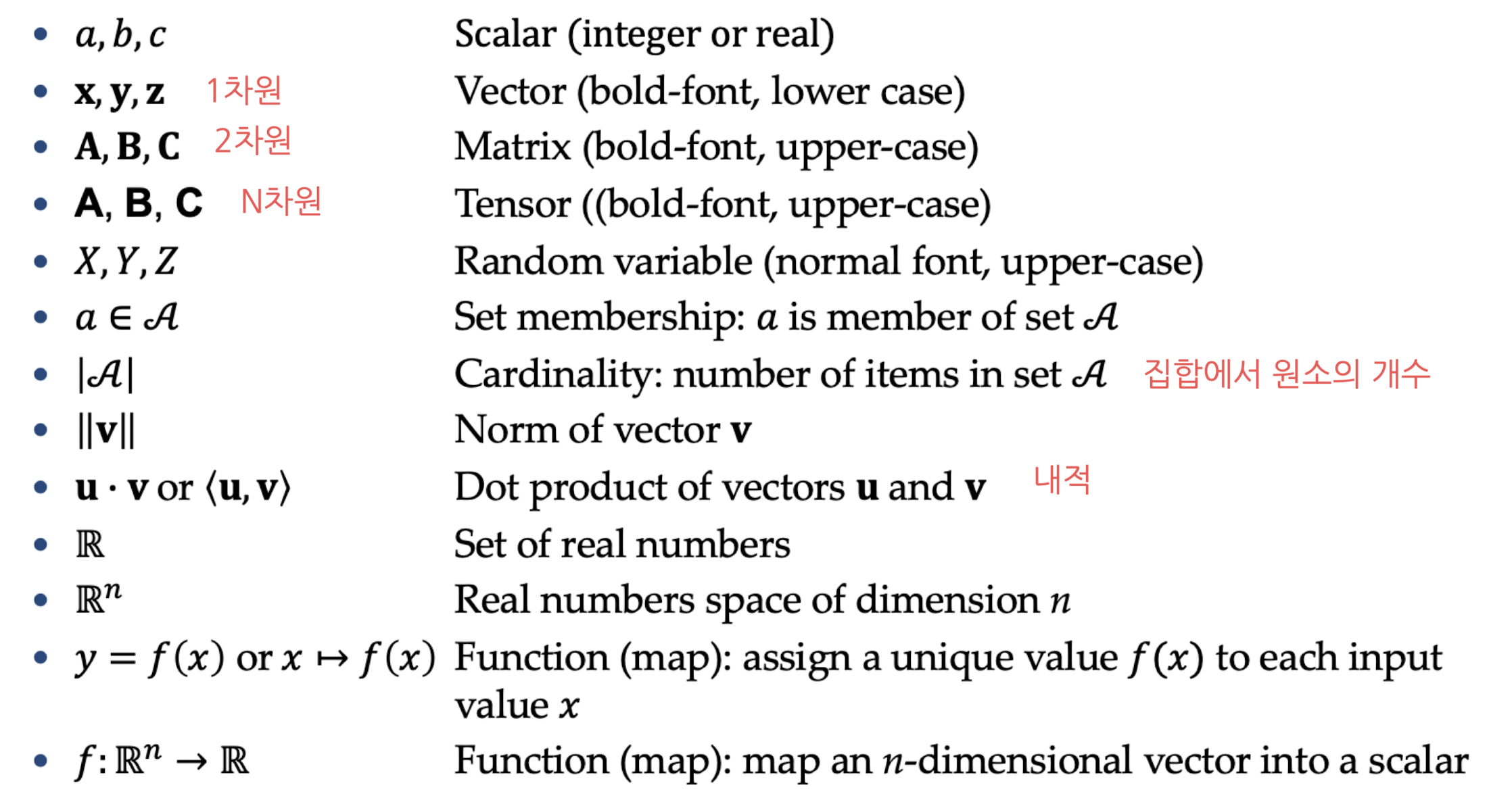
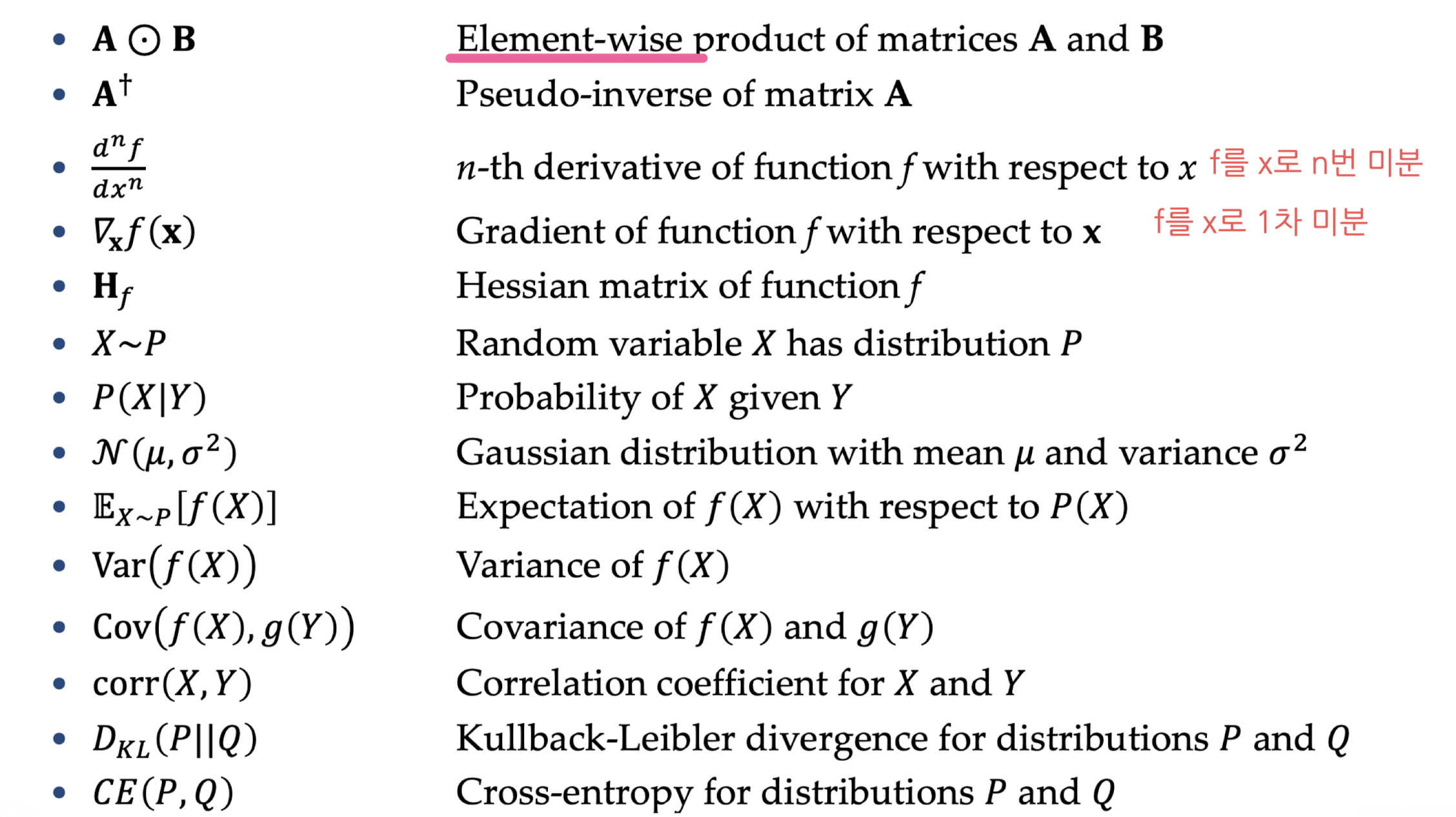
Notation
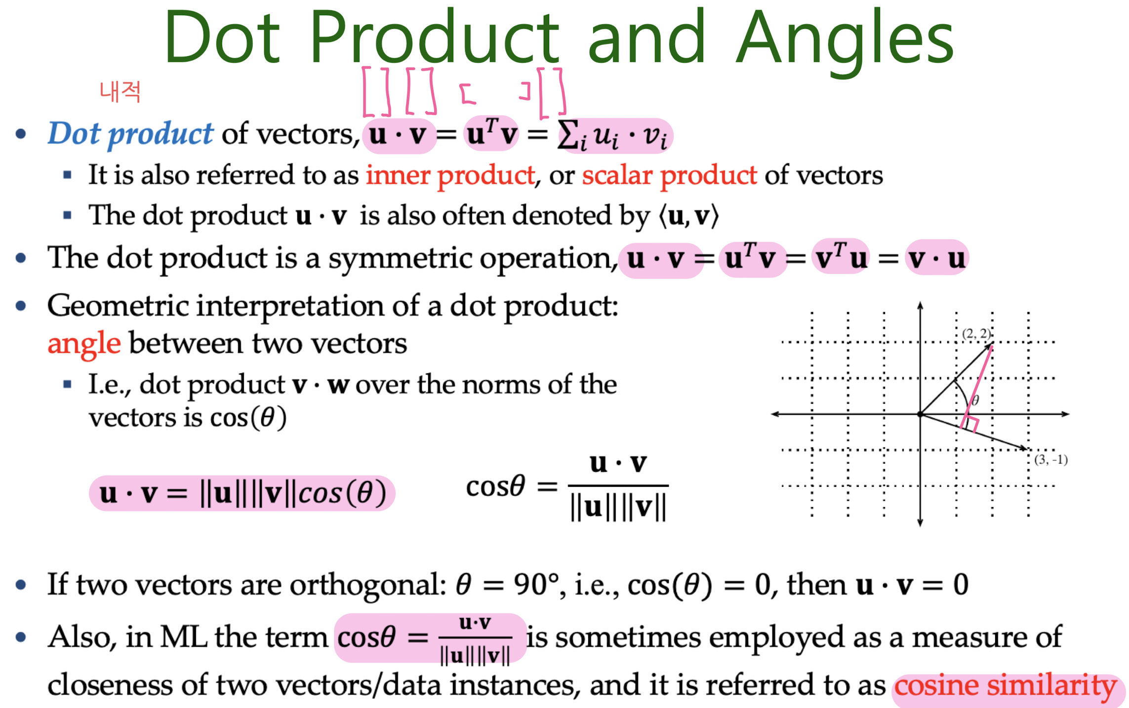
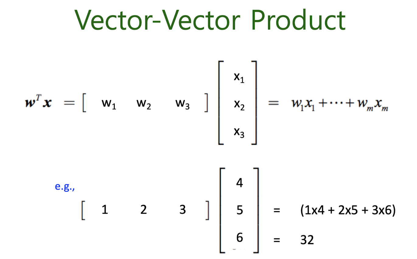
Dot Product and Angles
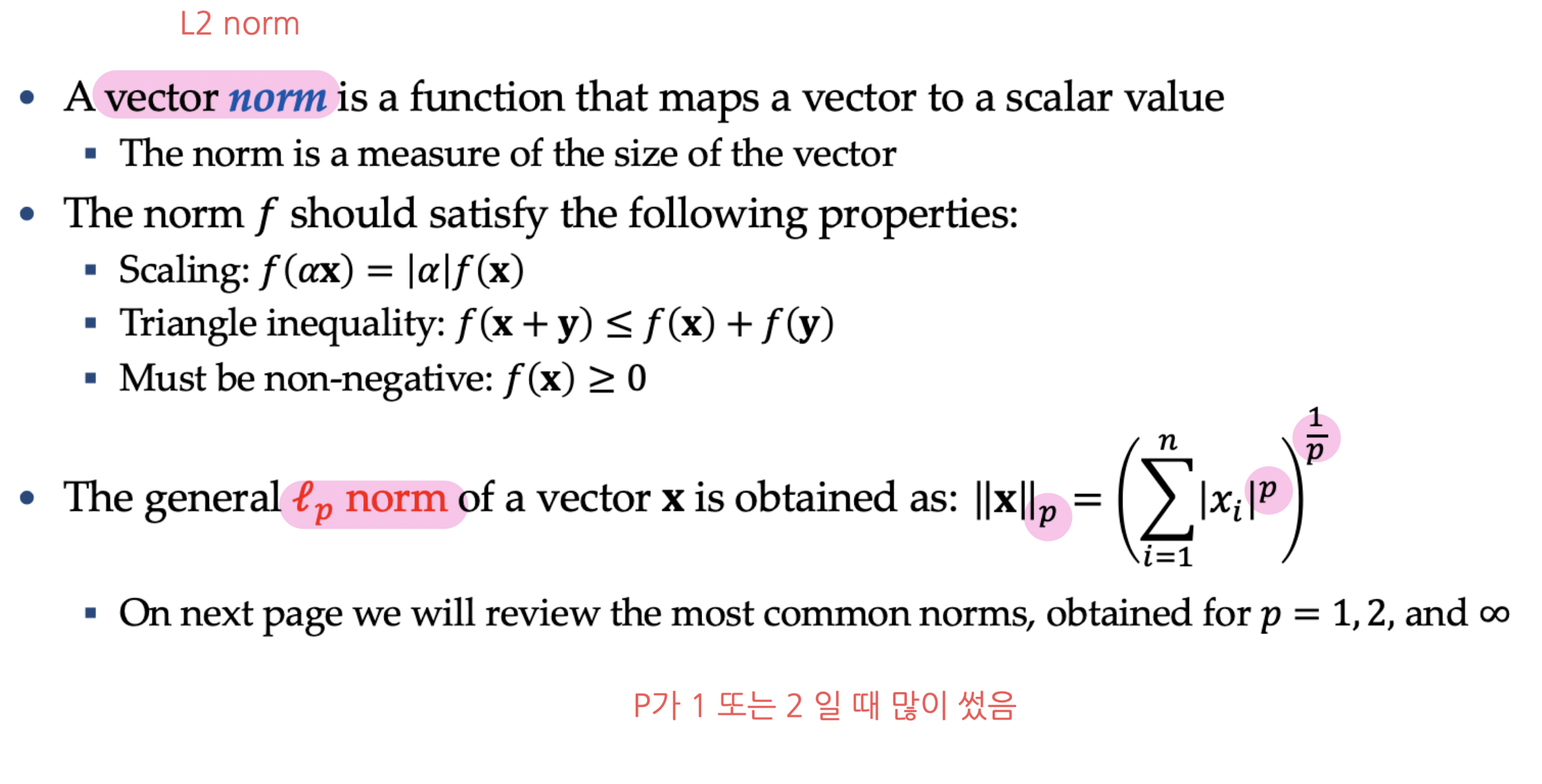
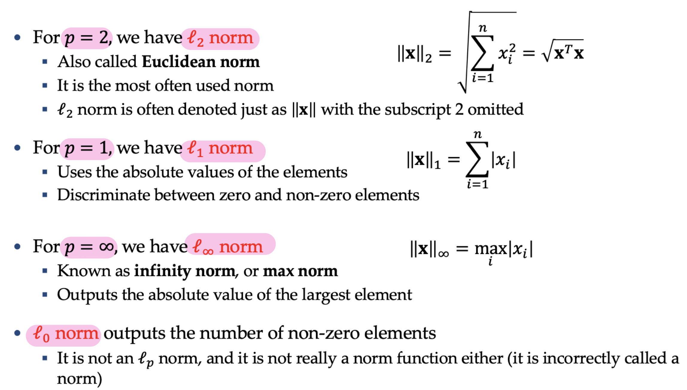
Norm of a Vector
Hyperlanes

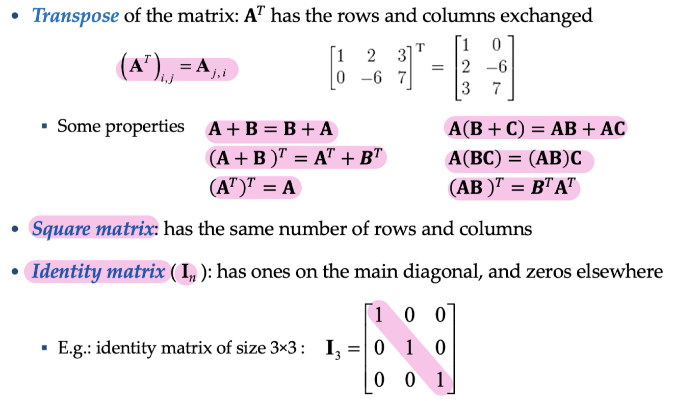
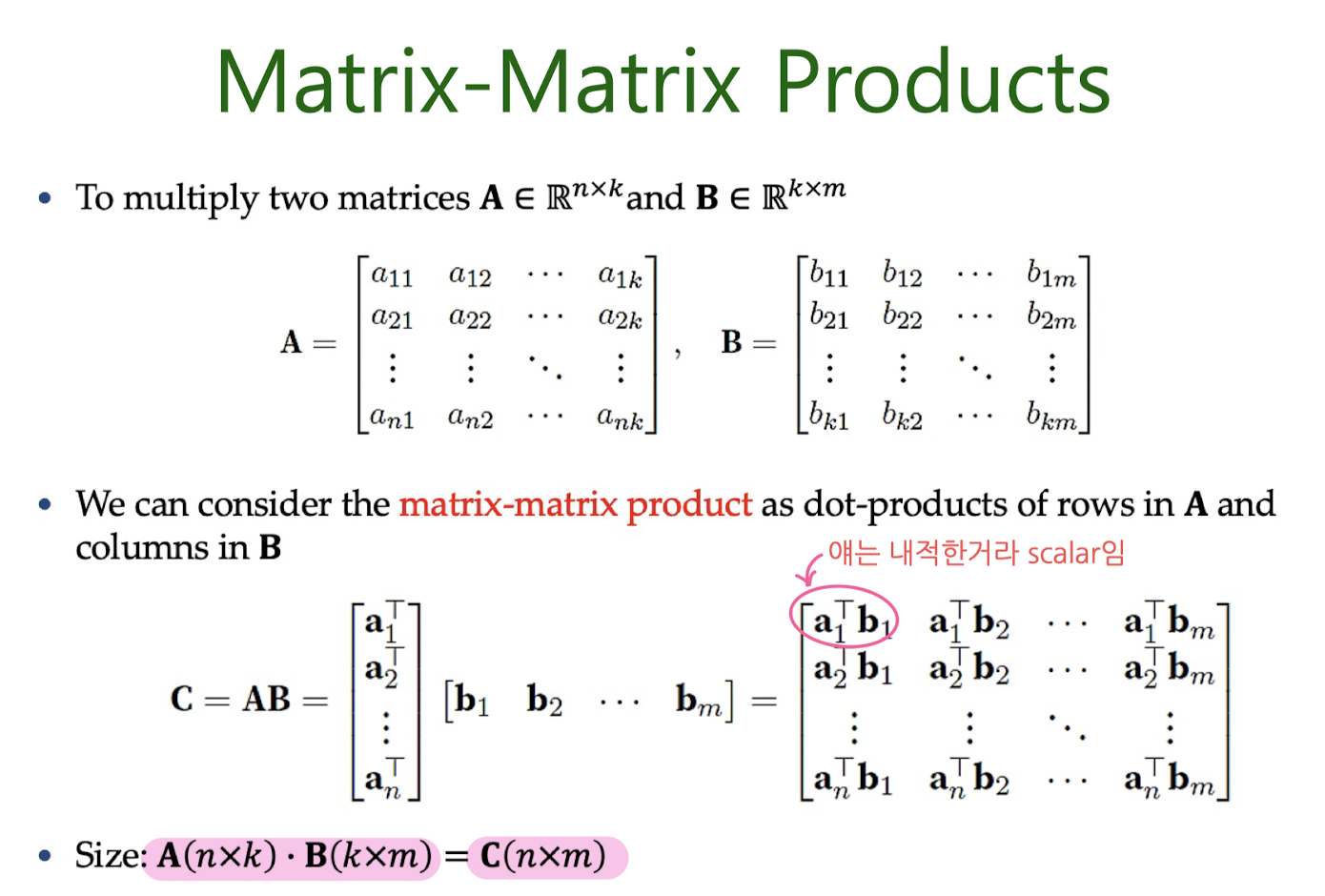
Matrics


Tensors
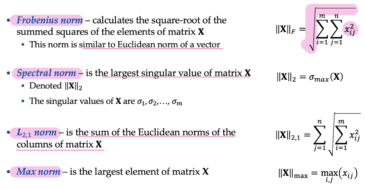
Matrix Norms
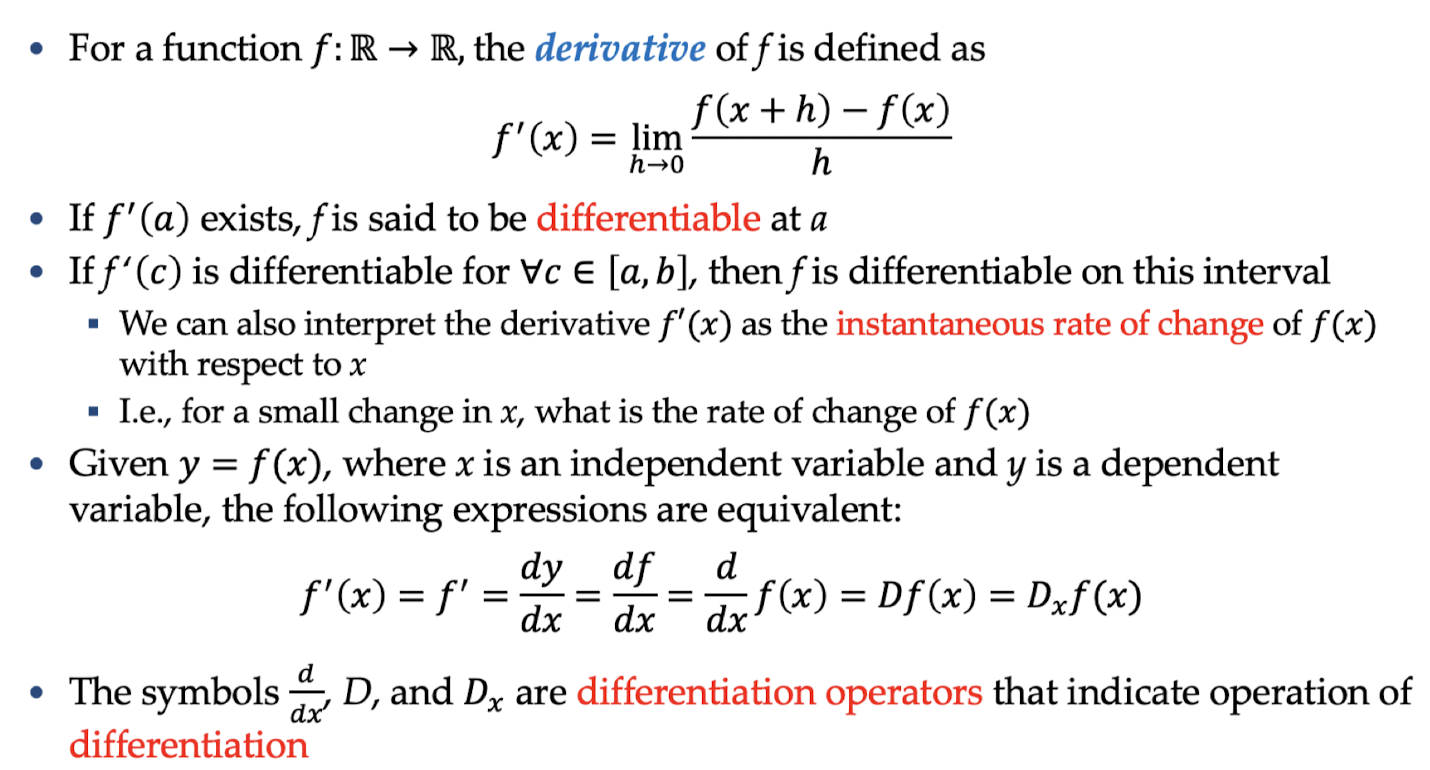
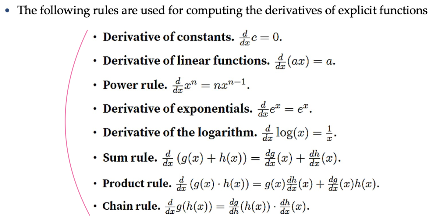
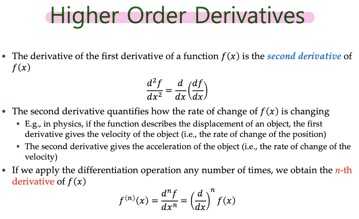
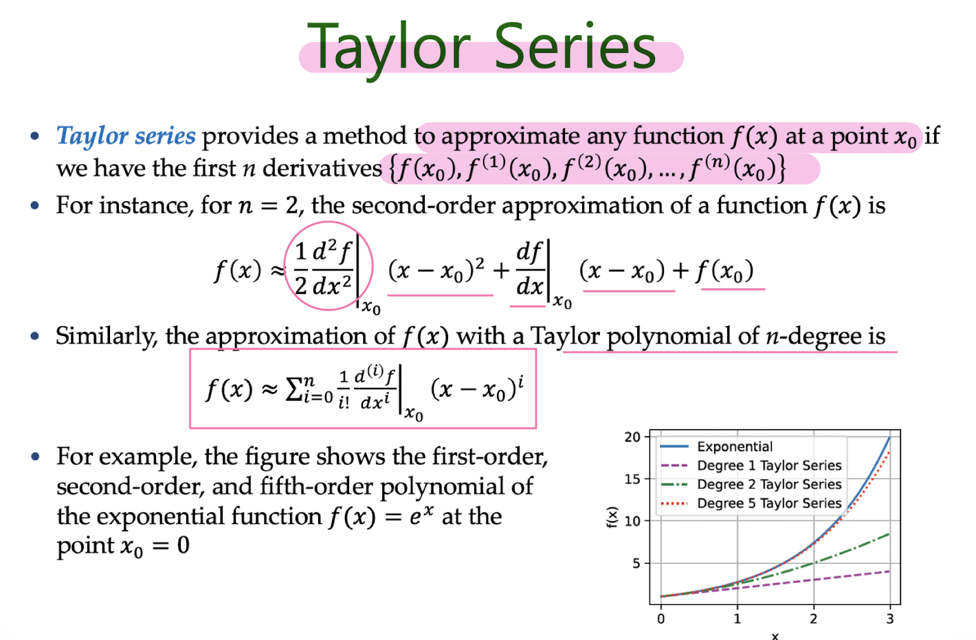
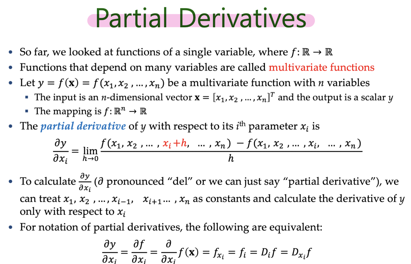
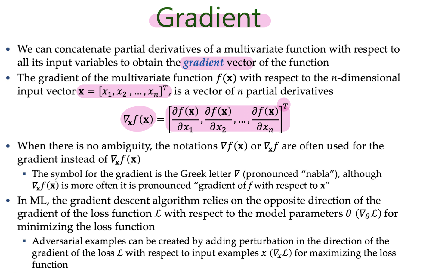
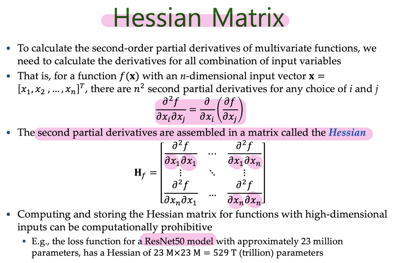
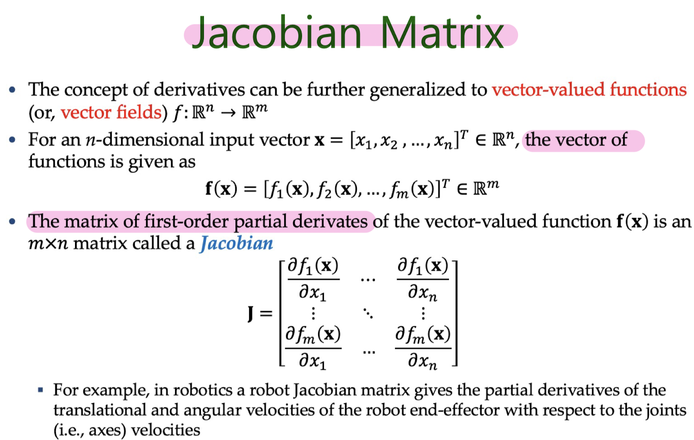
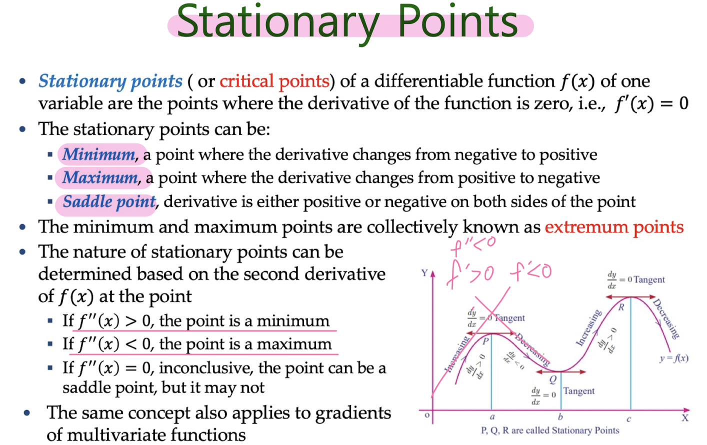
Differential Calculus
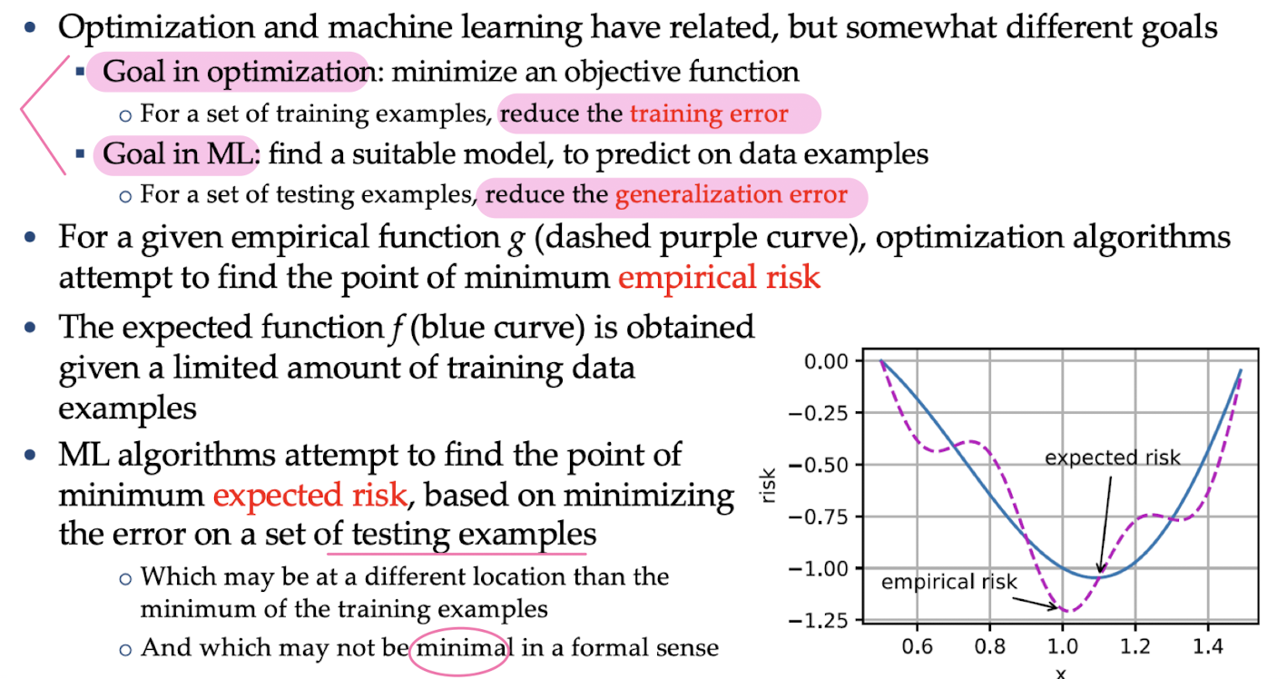
Optimization
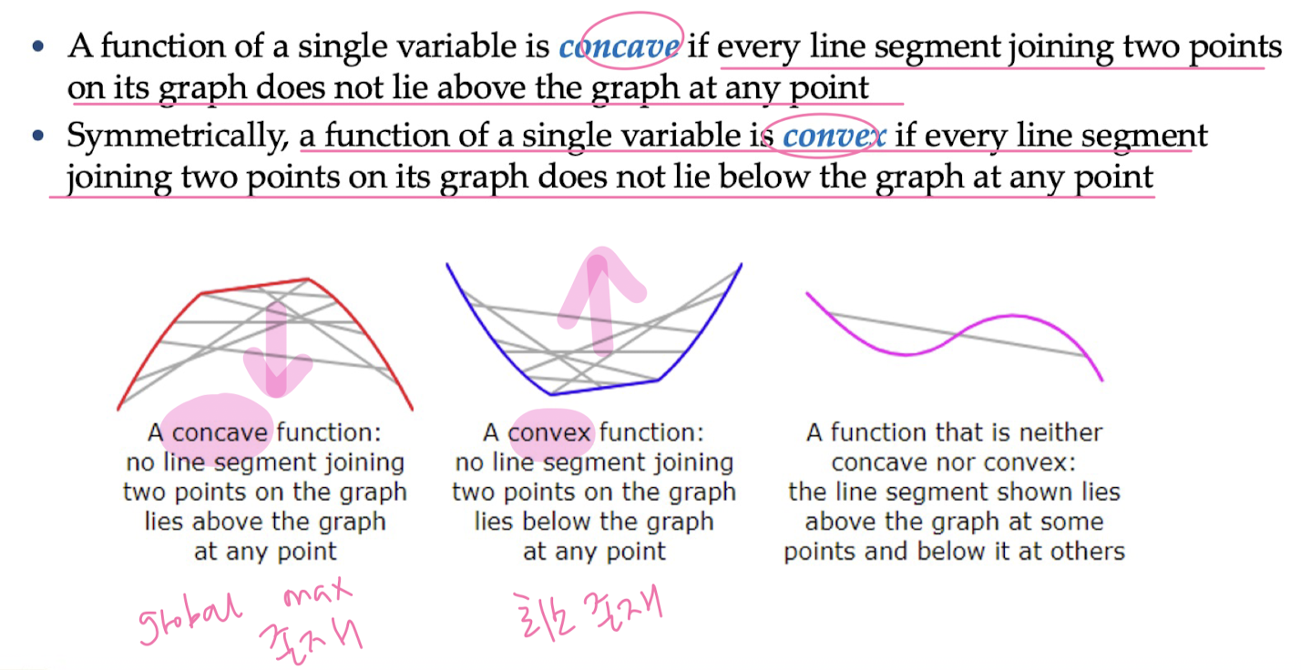
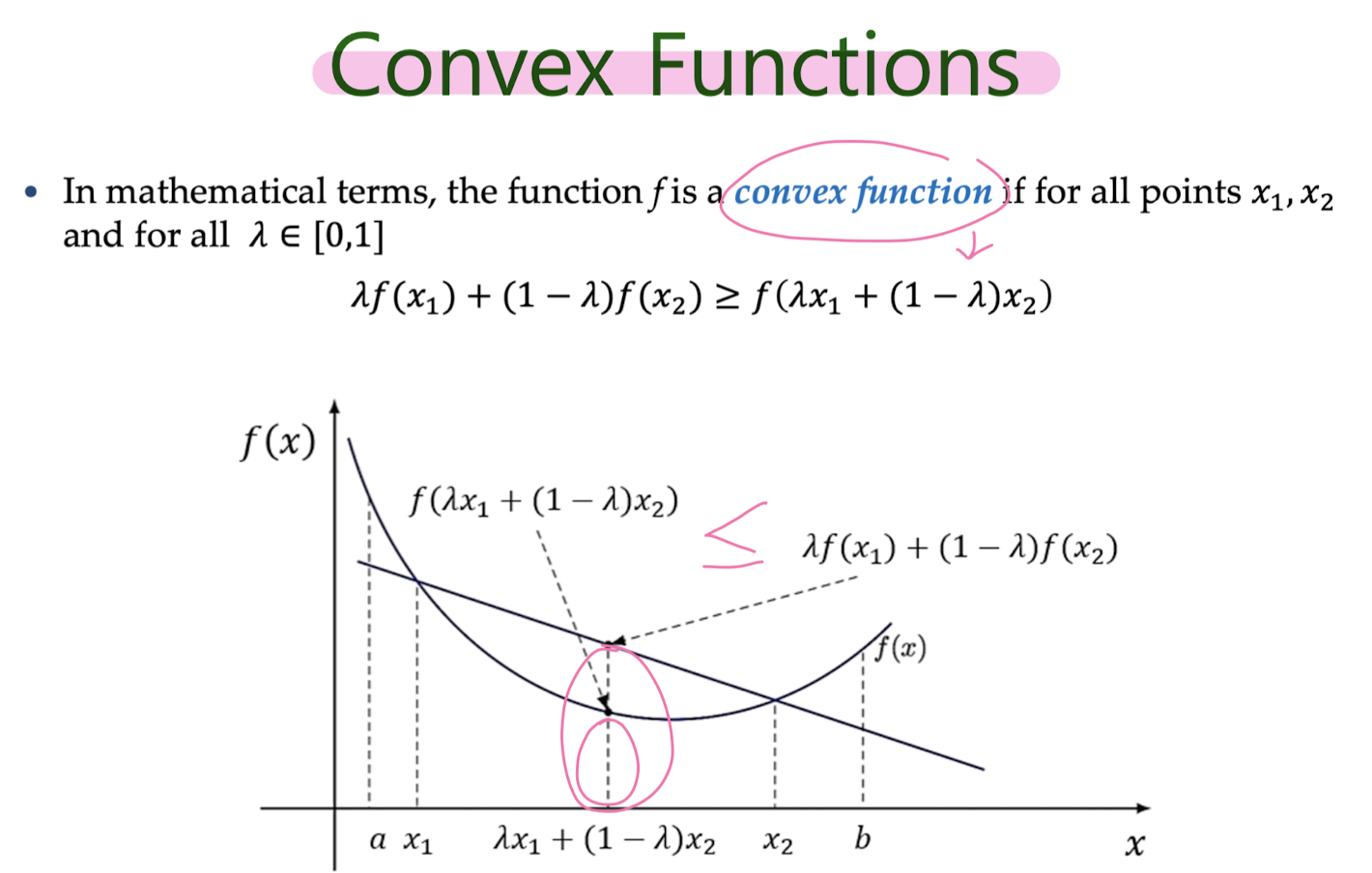
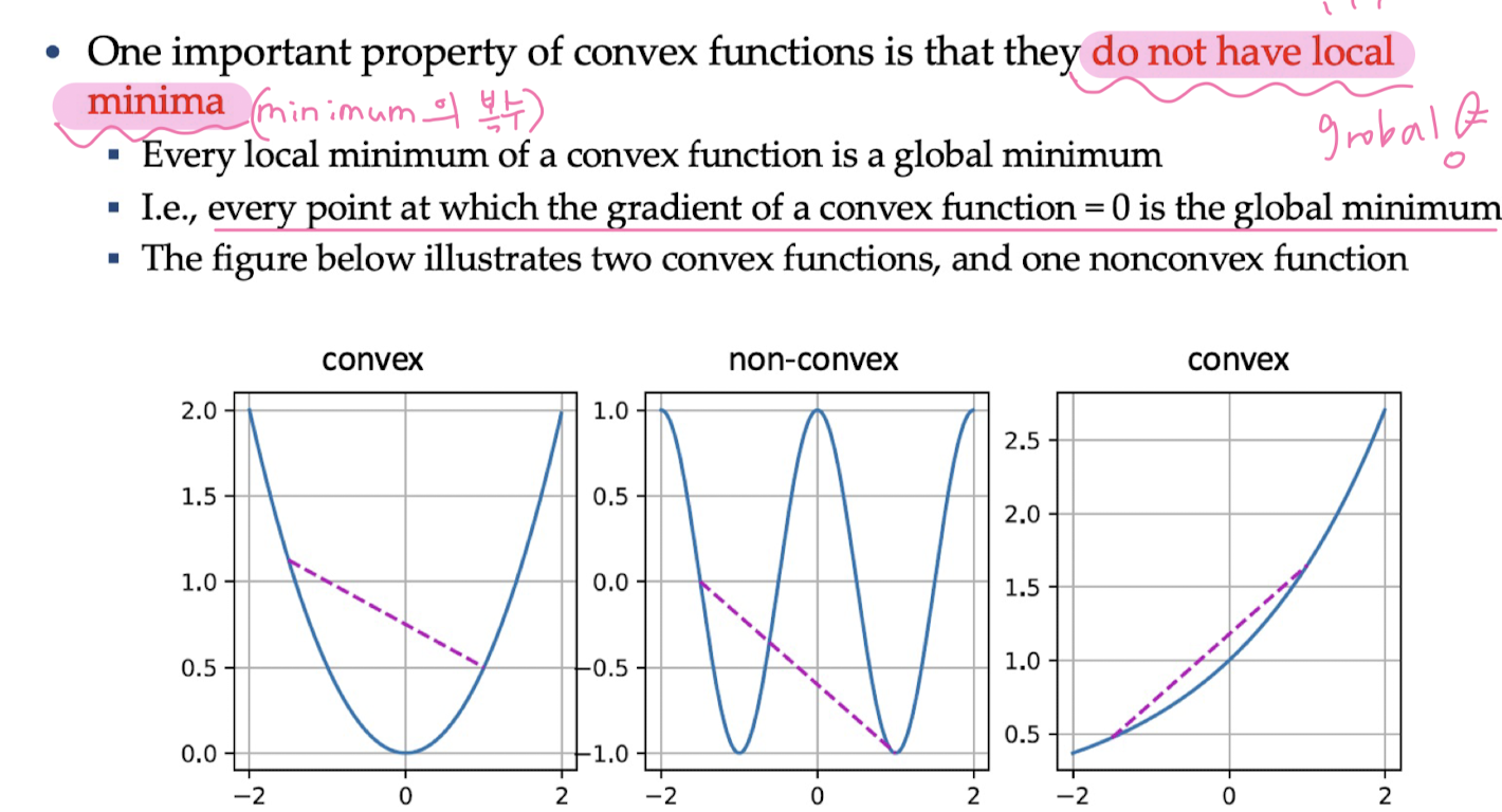
Convex Functions
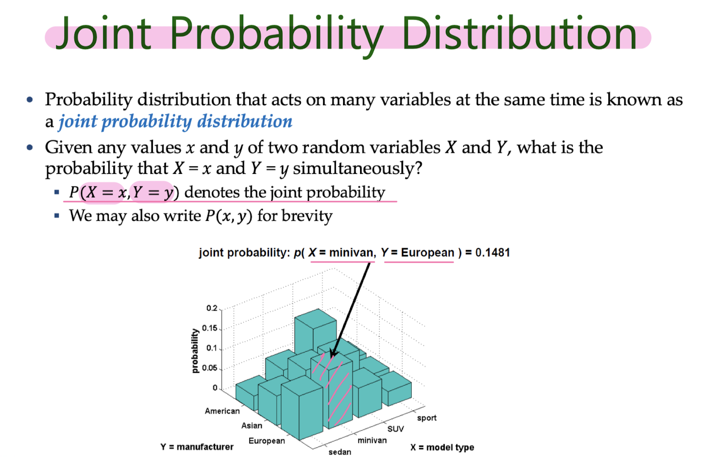
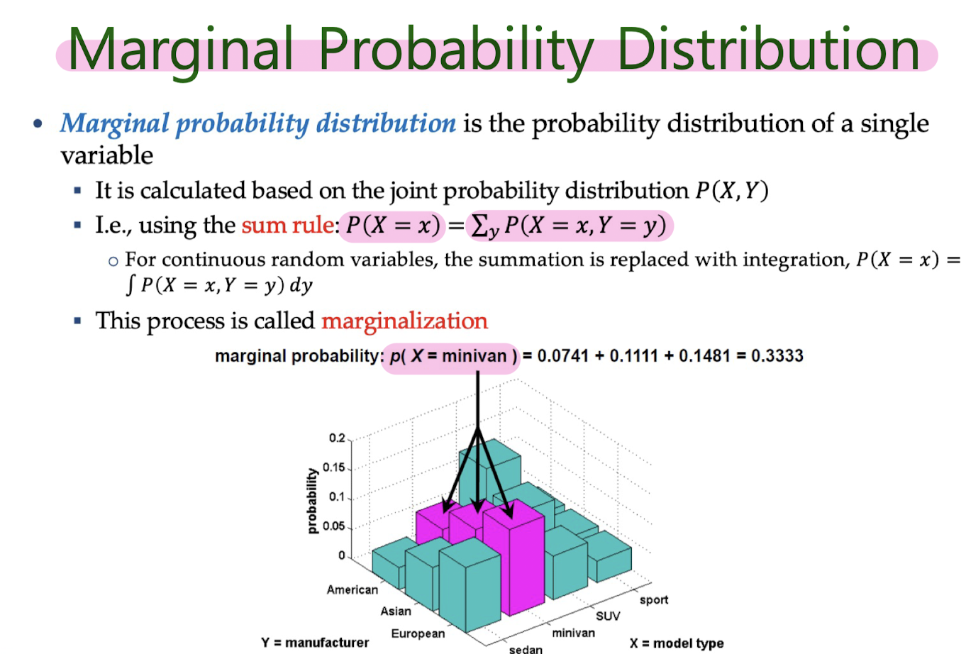
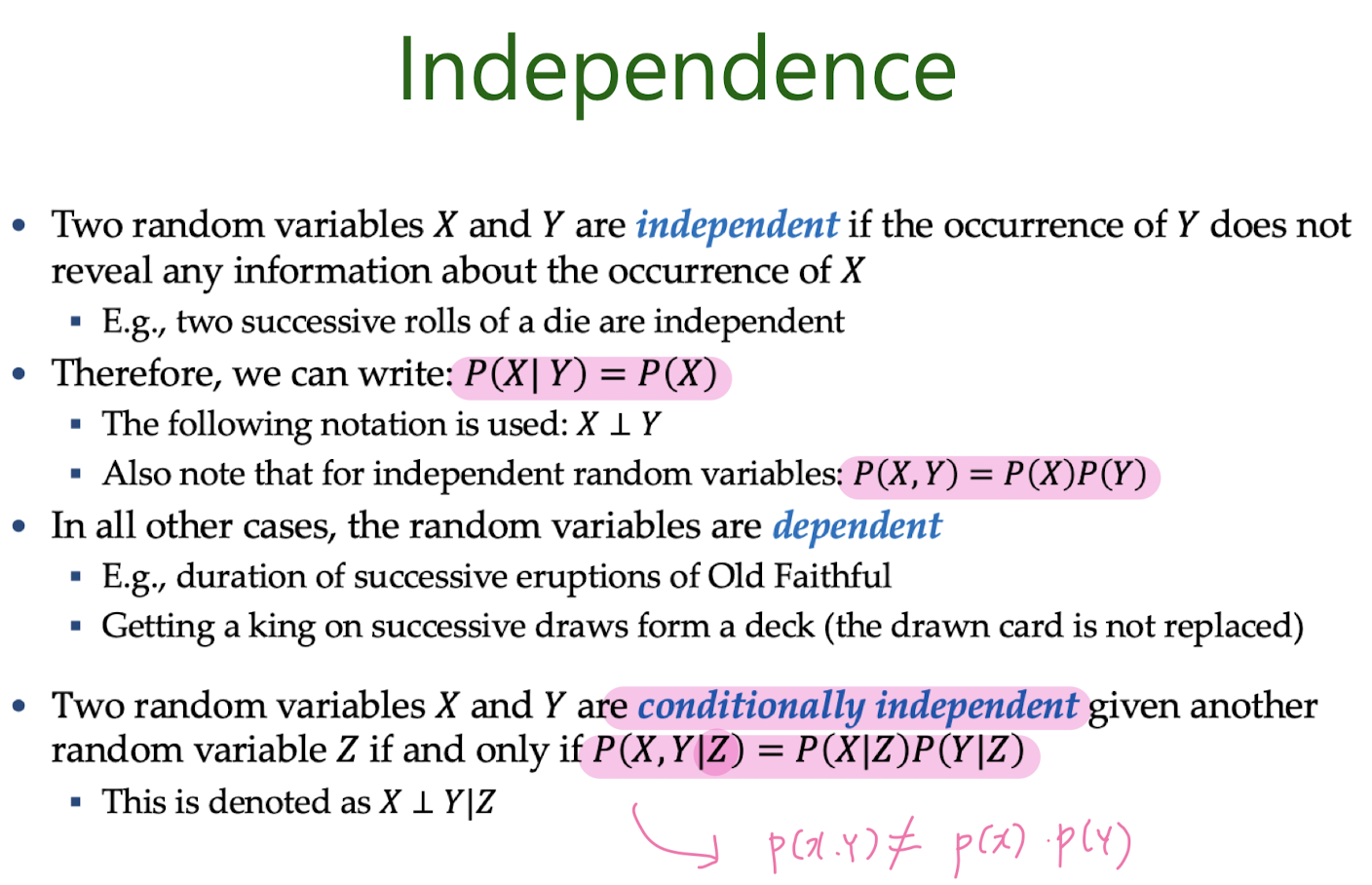
Probability
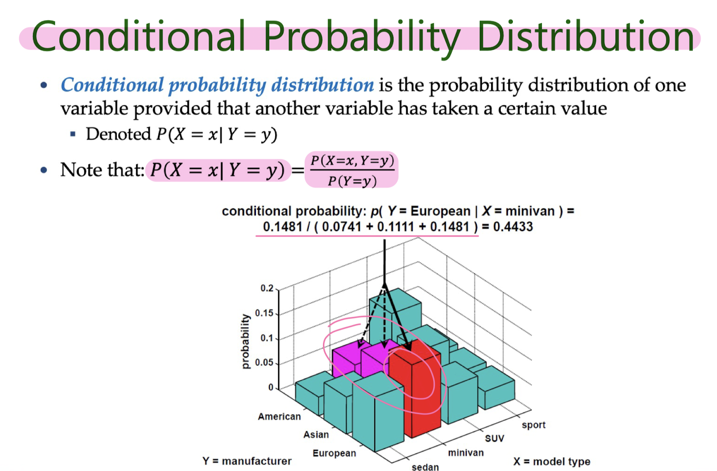
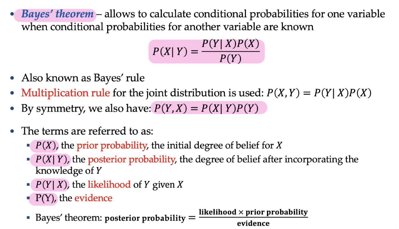
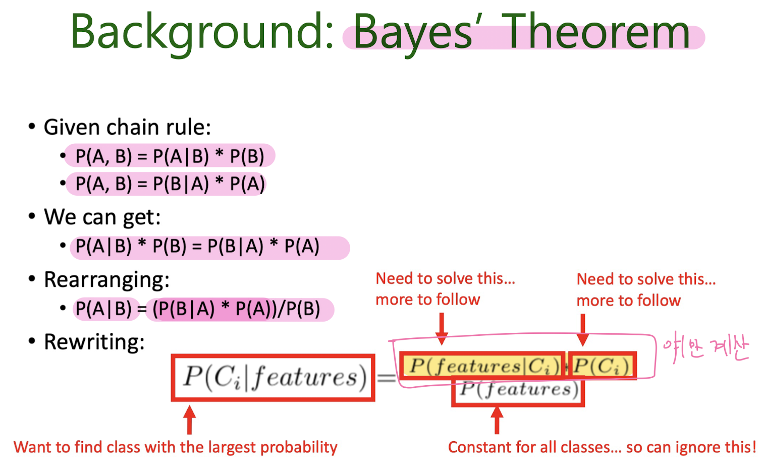
Bayes' Theorem
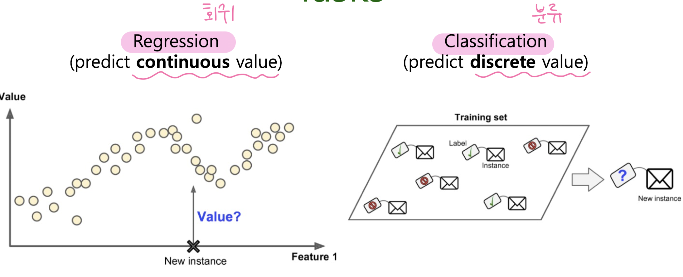
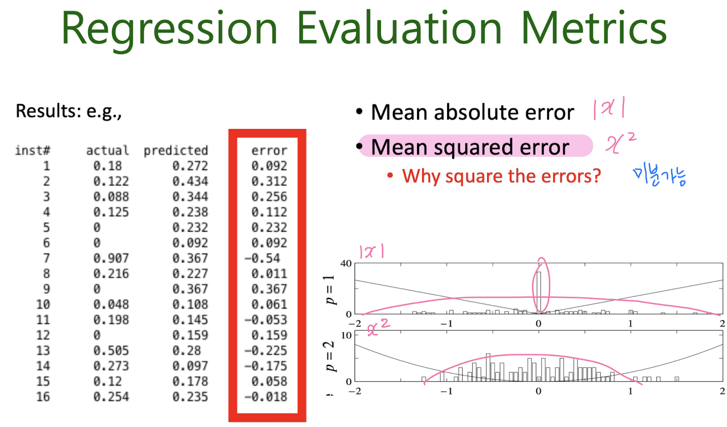
3. Regression
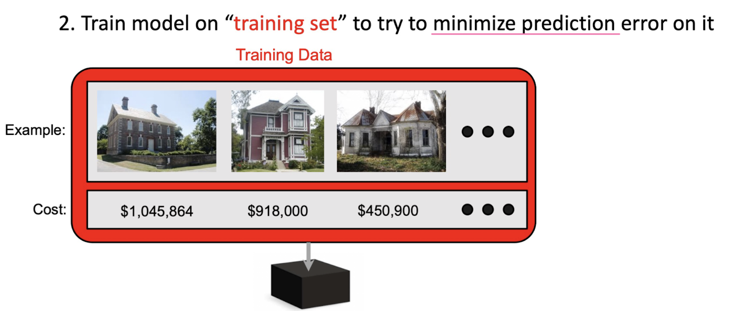
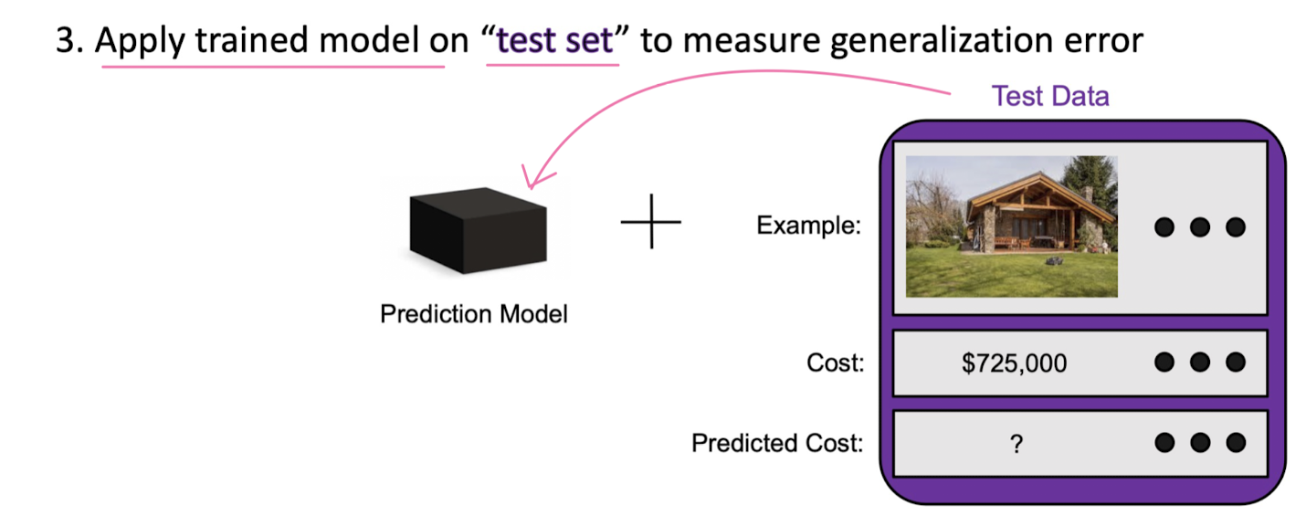
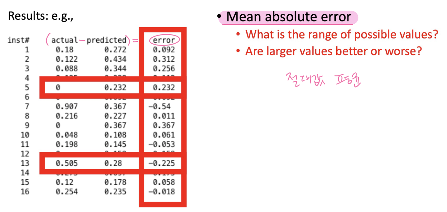
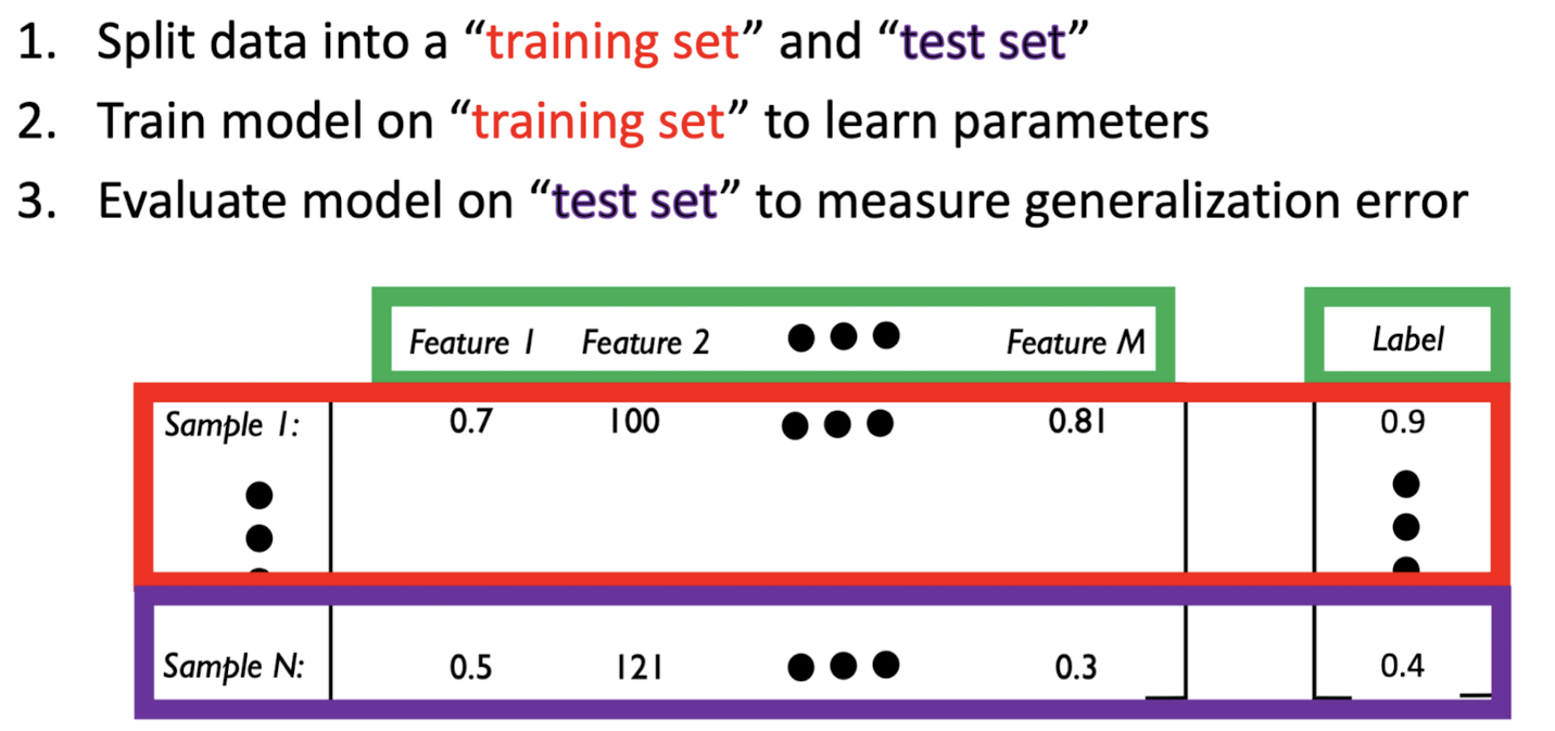
Evaluating regression models
regression evaluation metricss
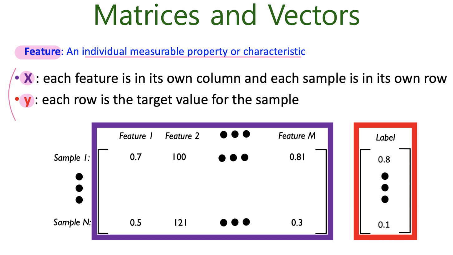
Background:Notation
3-1. Linear Regression
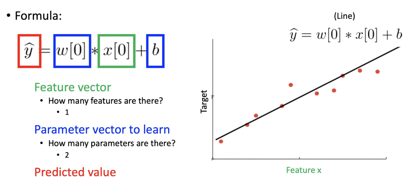
Simple Linear Regresstion Model
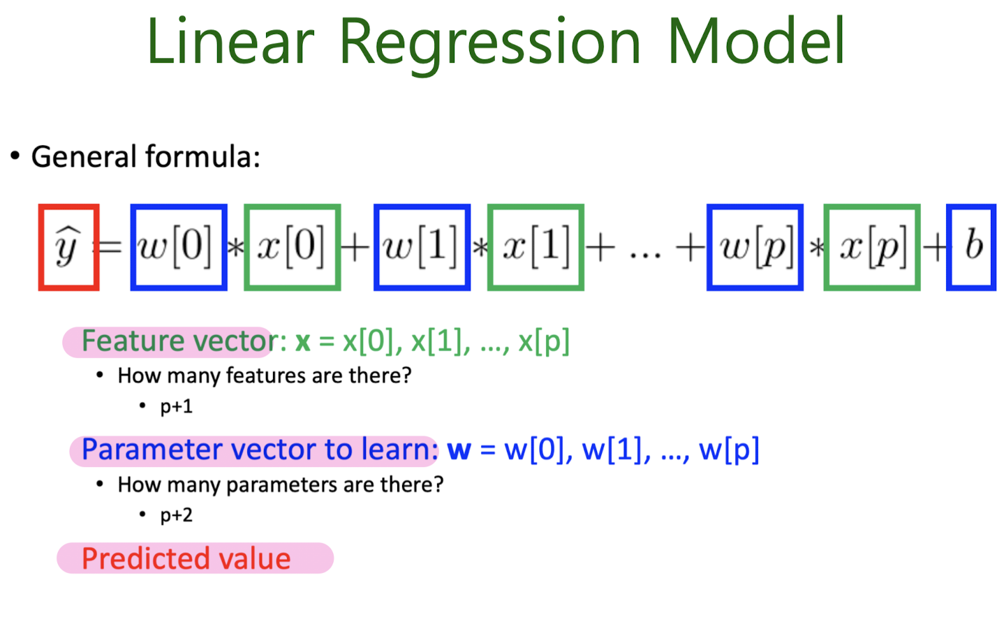
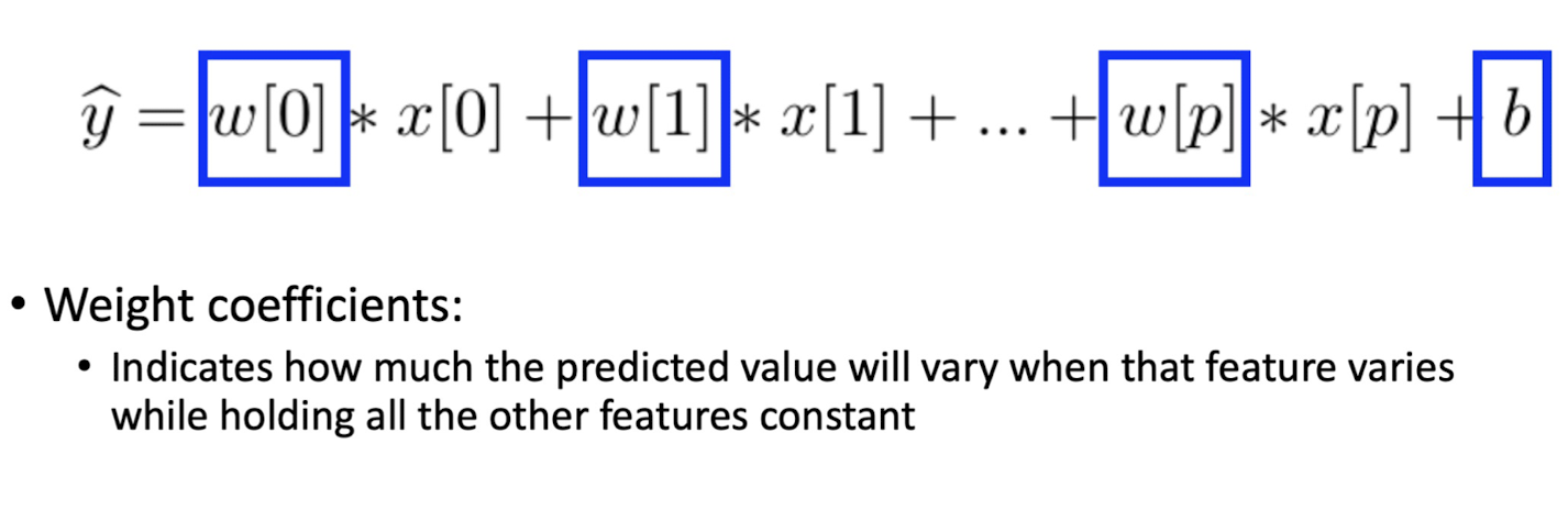
Mutiple Linear Regresstion Model
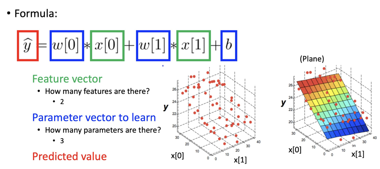
What to Learn?
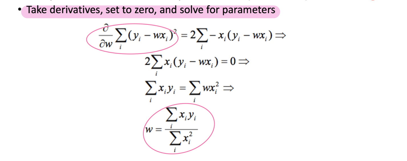
Learning Parameters
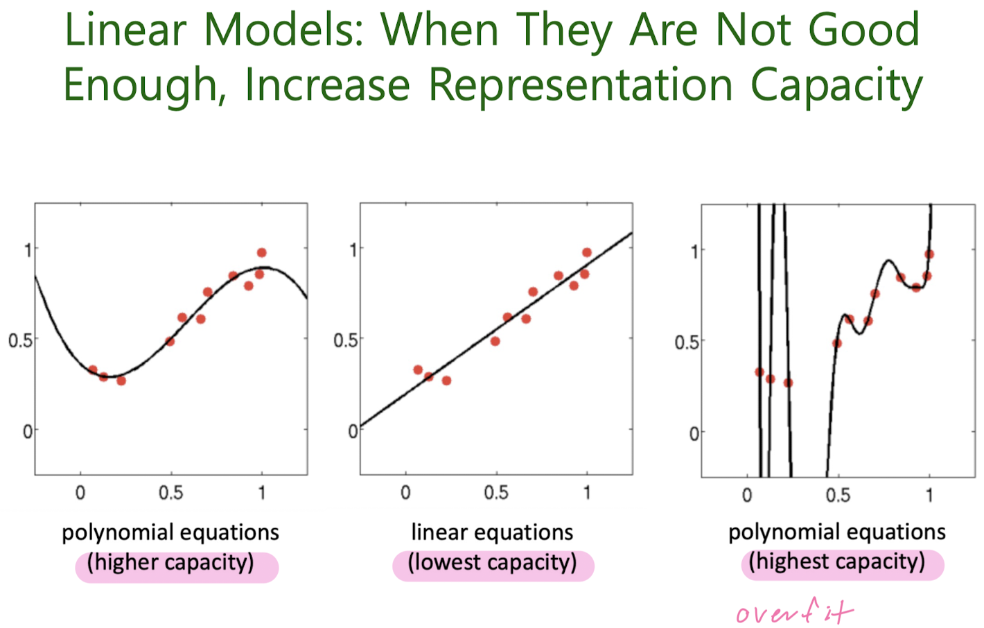
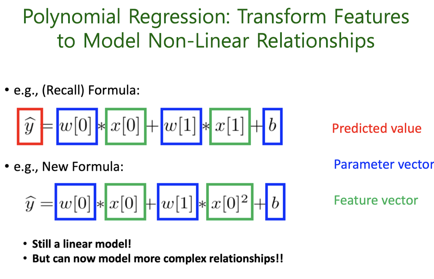
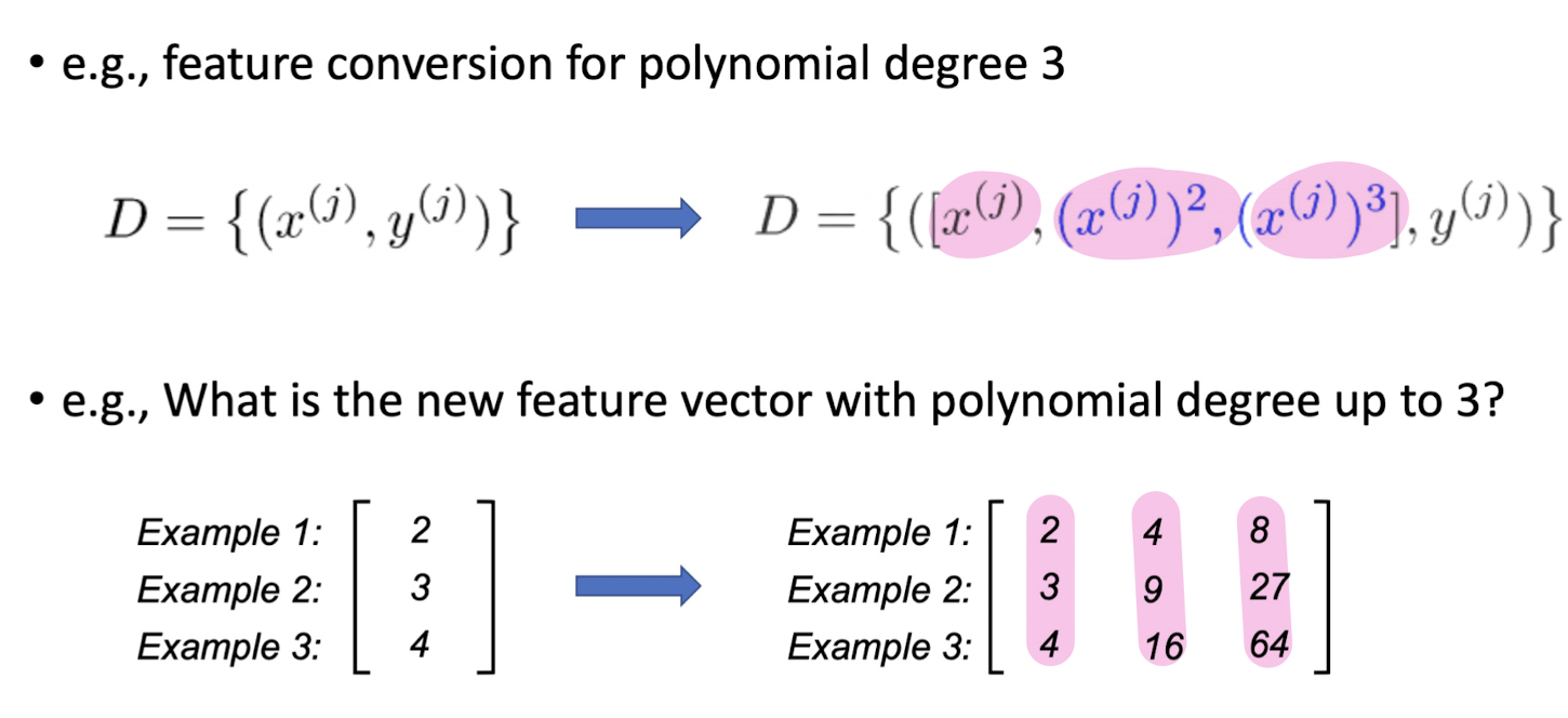
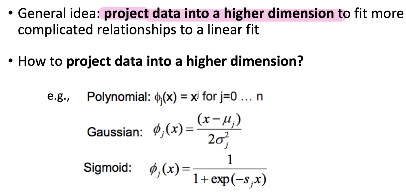
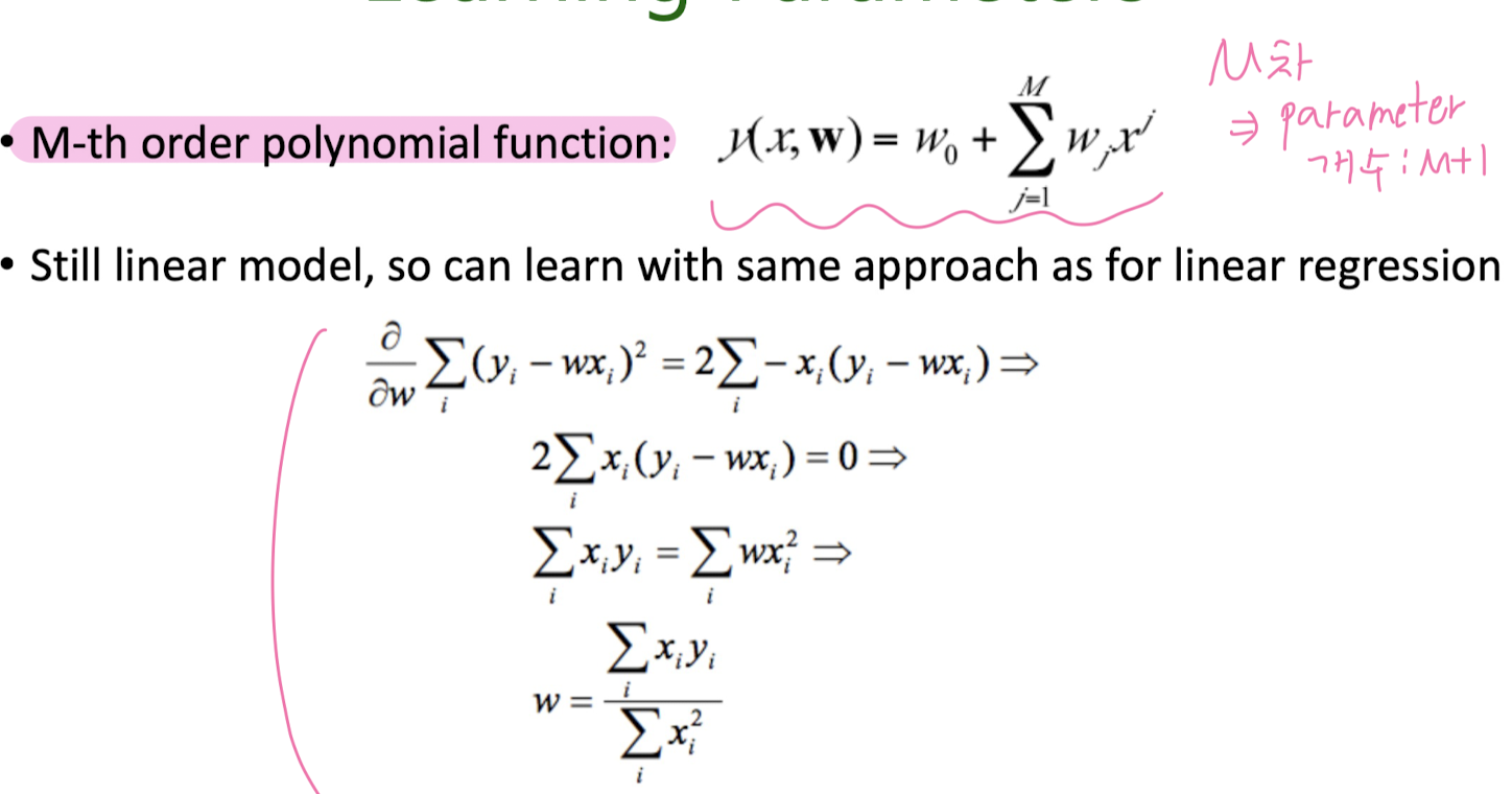
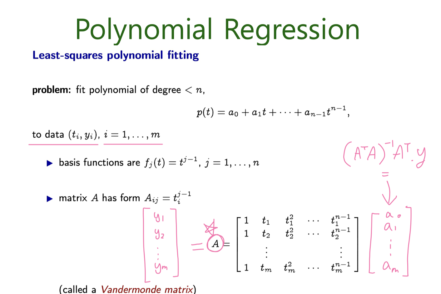
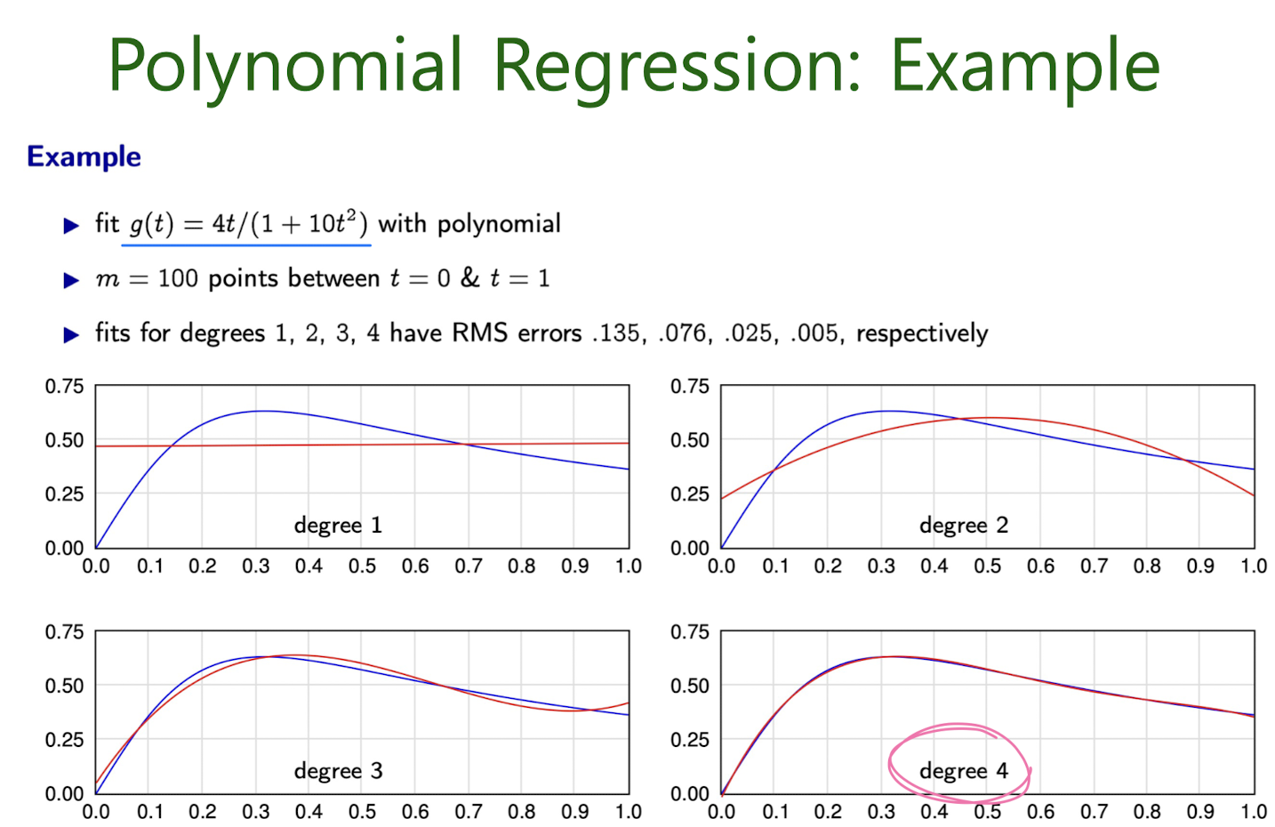
3-2. Polynomial Regression
Learning Parameters
What Feature Transformation to Use?

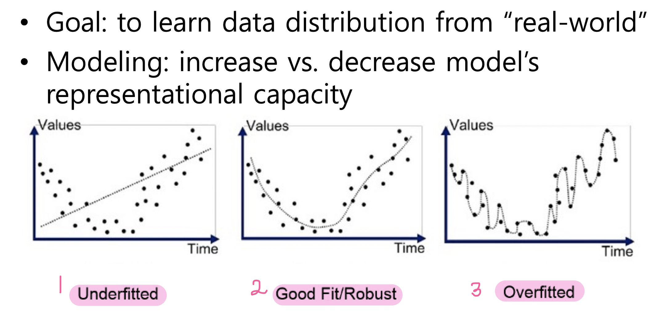
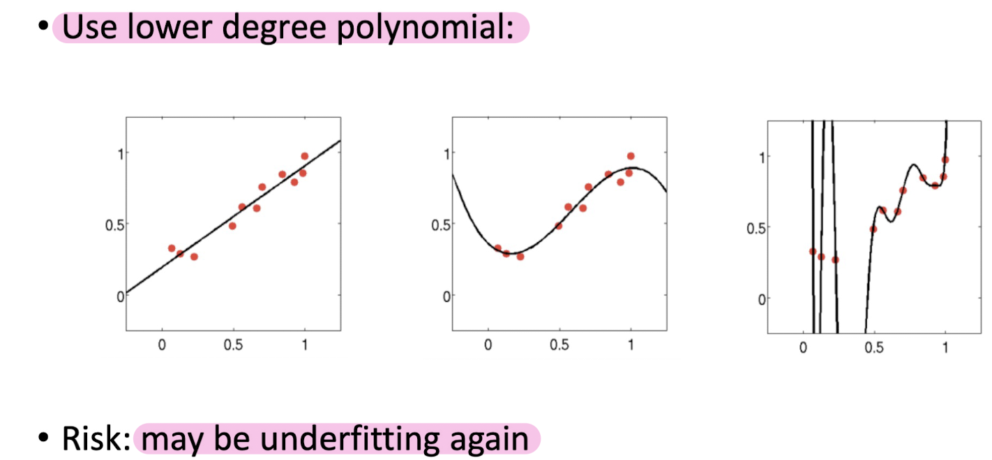
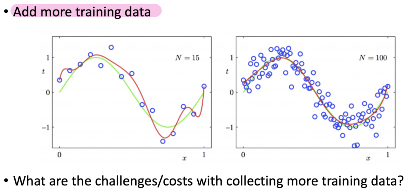
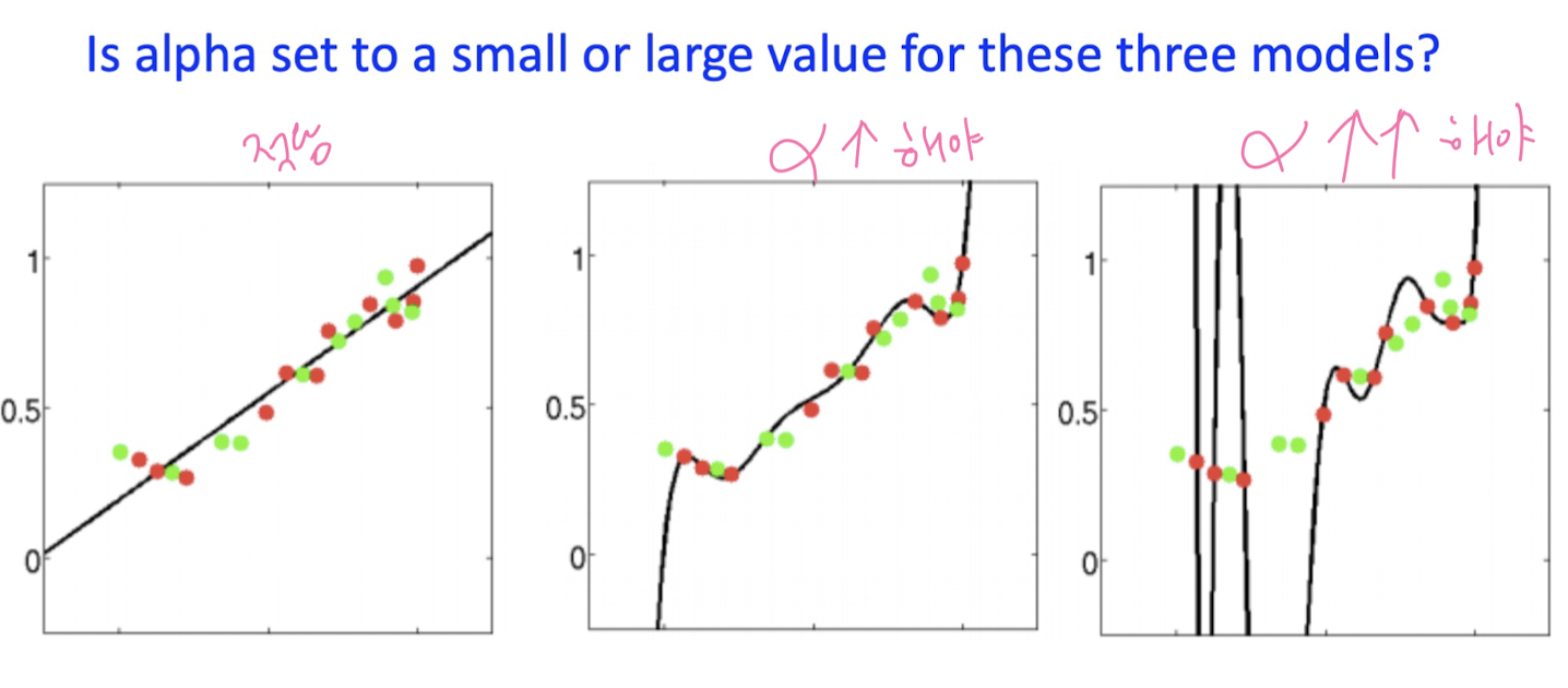
How to Avoid Overfitting

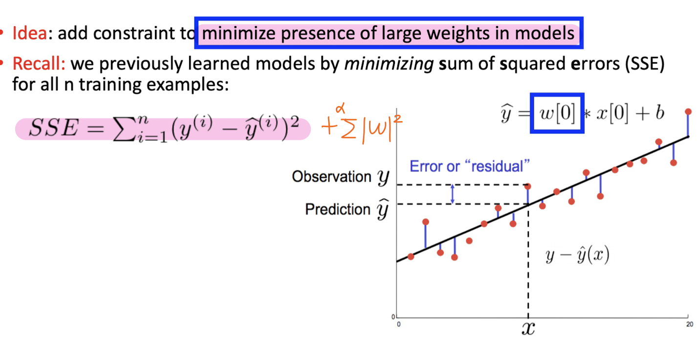
3-3. Regularization
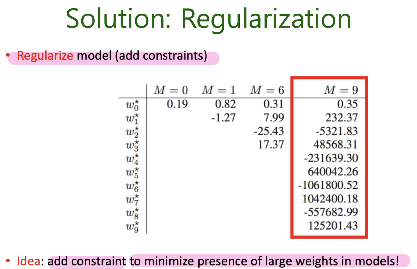
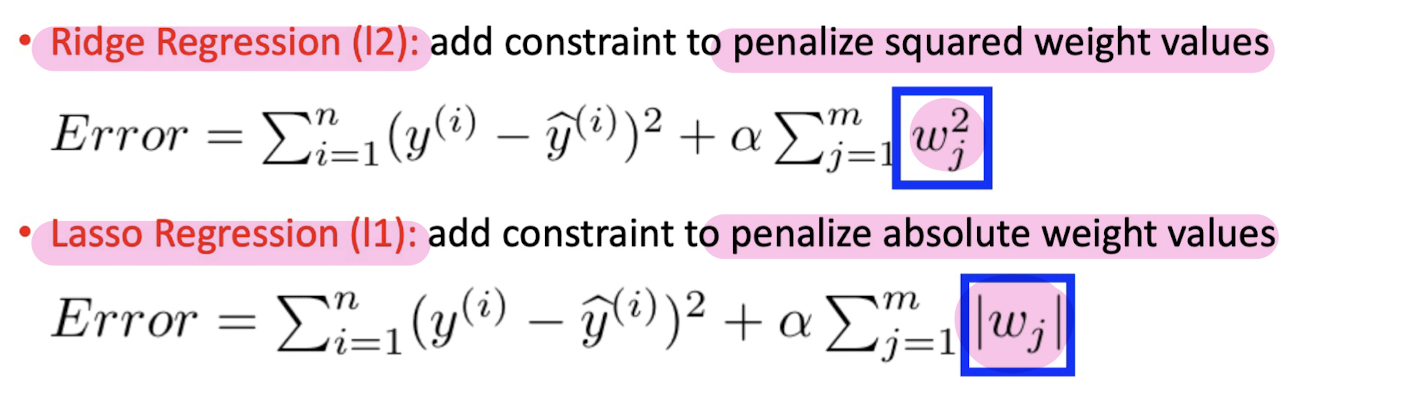
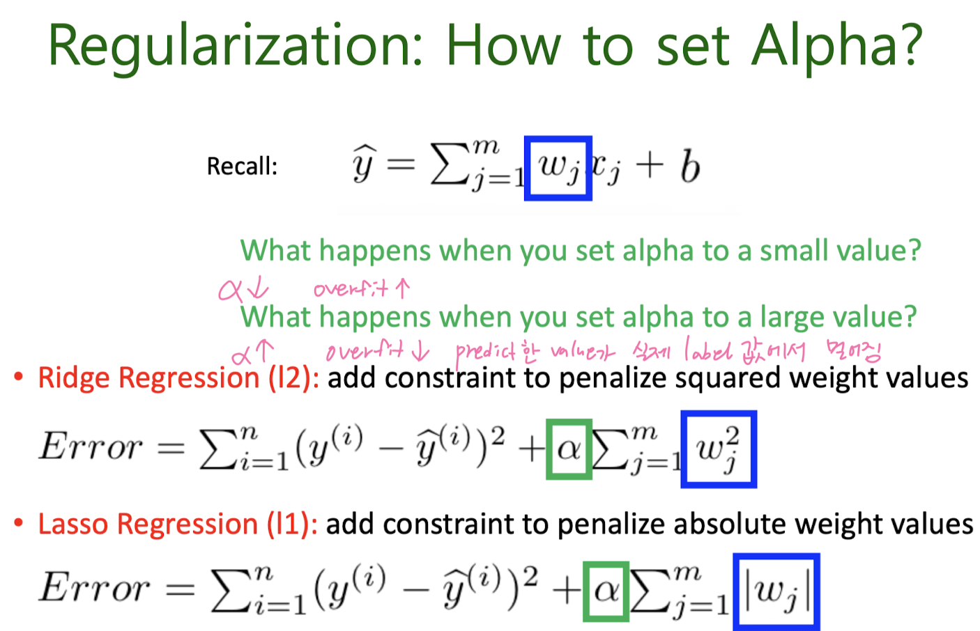
Ridge Regression / Lasso Regression
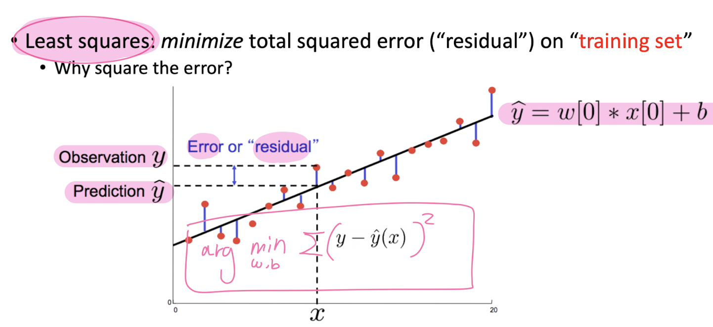
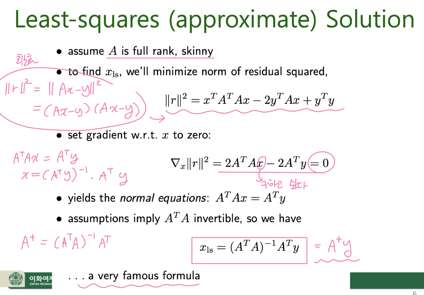
- Least-Squares Solution
최소 제곱 해결책은 모델이 관측된 목표 값과 모델에 의해 예측된 값 간의 제곱 차이의 합을 최소화하는 선형 회귀 모델의 매개변수(계수 또는 가중치)를 찾는 방법입니다. 리지 회귀(Ridge Regression)의 맥락에서는 정규화 항을 고려한 것입니다.
다음은 최소 제곱 해결책의 단계별 설명입니다.
-
선형 회귀 모델: 선형 회귀에서 입력 특성(독립 변수)을 행렬 X로, 목표 변수(종속 변수)를 벡터 y로 나타냅니다. 목표는 선형 모델
y = Xw가 데이터와 가능한 가깝게 일치하도록 가중치(일반적으로w로 표시)의 집합을 찾는 것입니다. -
목적 함수: 목적은 잔차 제곱합(RSS) 또는 평균 제곱 오차(MSE)를 최소화하는 것입니다. RSS는 실제 목표 값과 예측 값 사이의 제곱 차이의 합으로 정의됩니다.
RSS(w) = Σ(yᵢ - Xᵢw)²여기서:
yᵢ는 i번째 관측된 목표 값입니다.Xᵢ는 특성 행렬 X의 i번째 행입니다.w는 가중치(계수) 벡터입니다.
-
최소 제곱 해결책: RSS를 최소화하는 가중치
w를 찾기 위해 RSS를w에 대해 미분하고 그 값을 0으로 설정합니다. 이 방정식을 해결하면 최소 제곱 해결책이 나옵니다.XᵀXw = Xᵀy여기서:
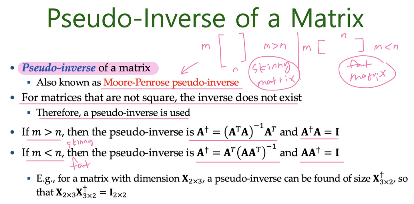
Xᵀ는 특성 행렬 X의 전치입니다.XᵀX는 X의 전치와 X의 행렬 곱입니다.Xᵀy는 X의 전치와 목표 벡터 y의 행렬 곱입니다.
-
w를 구하기: 위의 방정식을 사용하여
w를 구할 수 있습니다.w에 대한 공식은 다음과 같습니다.w = (XᵀX)⁻¹ Xᵀy여기서
(XᵀX)⁻¹는XᵀX의 역행렬을 나타냅니다. 이 공식은 RSS를 최소화하는 가장 적합한 선형 회귀 모델의 가중치를 제공합니다. -
리지 회귀 수정: 리지 회귀에서는 목적 함수에 정규화 항을 추가하여 사용합니다. 정규화 항은 가중치
w의 크기를 제어함으로써 오버피팅을 방지합니다. 리지 회귀의 목적 함수는 다음과 같이 정의됩니다.J(w) = ||y - Xw||² + α||w||²리지 회귀의 최소 제곱 해결책은 이 수정된 목적 함수를 최소화하는 가중치를 찾는 것입니다. 리지 회귀에서
w에 대한 공식은 다음과 같이 변합니다.w = (XᵀX + αI)⁻¹ Xᵀy여기서
I는 항등 행렬(identity matrix)입니다.
요약하면, 최소 제곱 해결책은 관측 값과 예측 값 간의 제곱 차이의 합을 최소화하는 선형 회귀 모델의 가중치를 찾는 수학적인 방법입니다. 리지 회귀에서는 정규화 항을 목적 함수에 추가하여 가중치의 크기를 제어하며, 모델 적합과 정규화를 균형있게 고려하는 수정된 목적 함수를 최소화하는 가중치를 찾습니다.
Review
Overdetermined Linear Equations
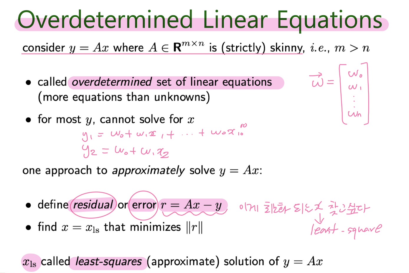
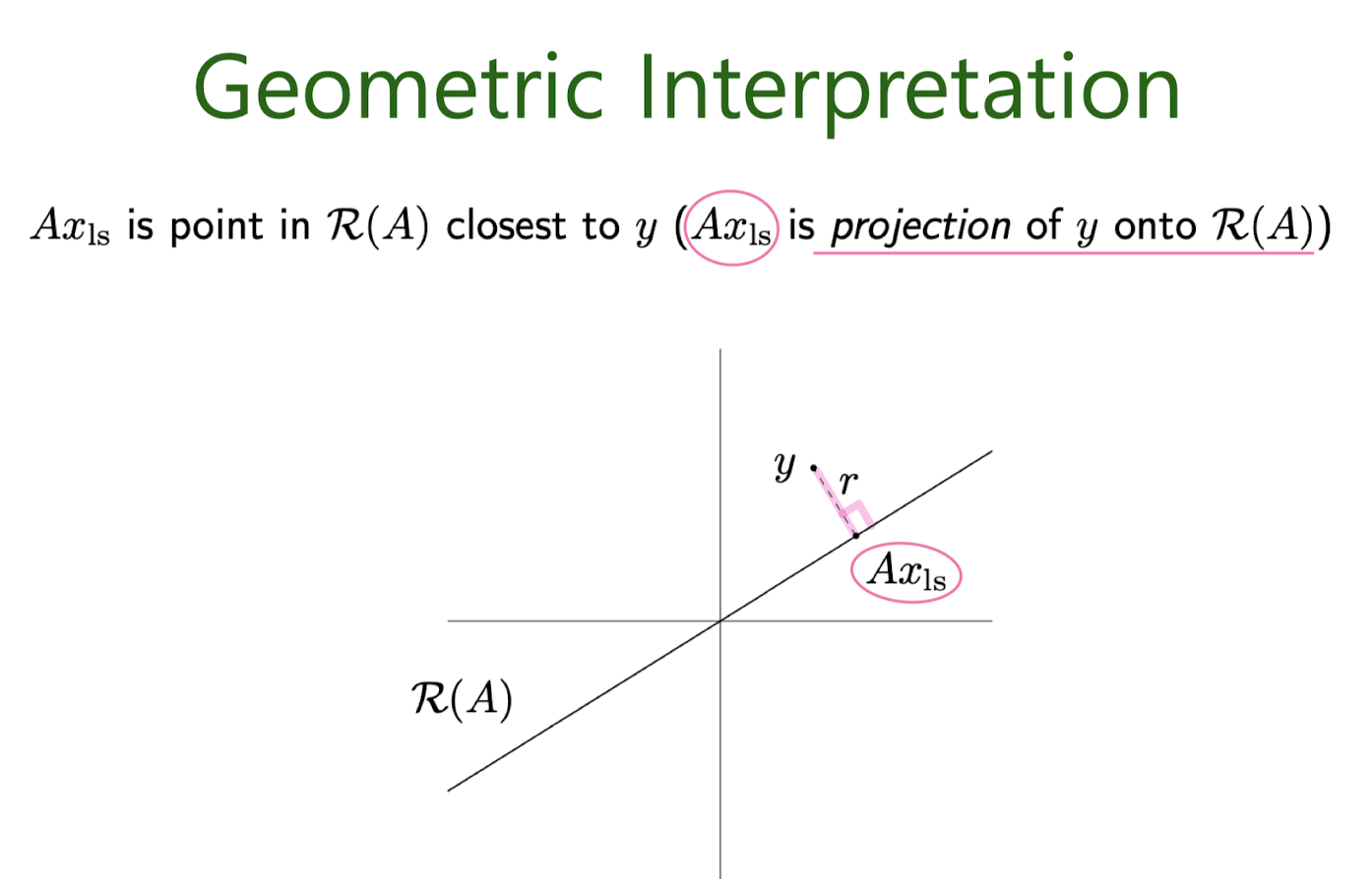
Least-Squares Solution

Polynomial Regressiion
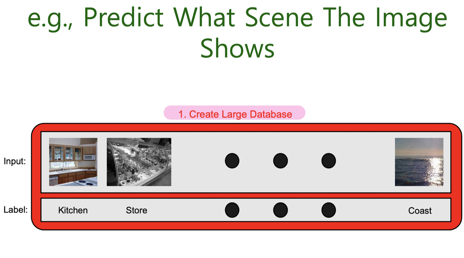
4. Classification : KNN, Decision tree
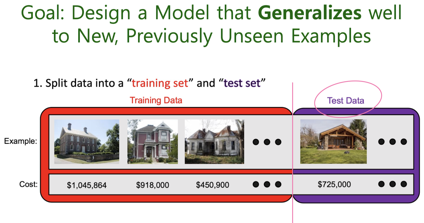
Goal: Design Models that Generalize Well to New, Previously Unseen Examples
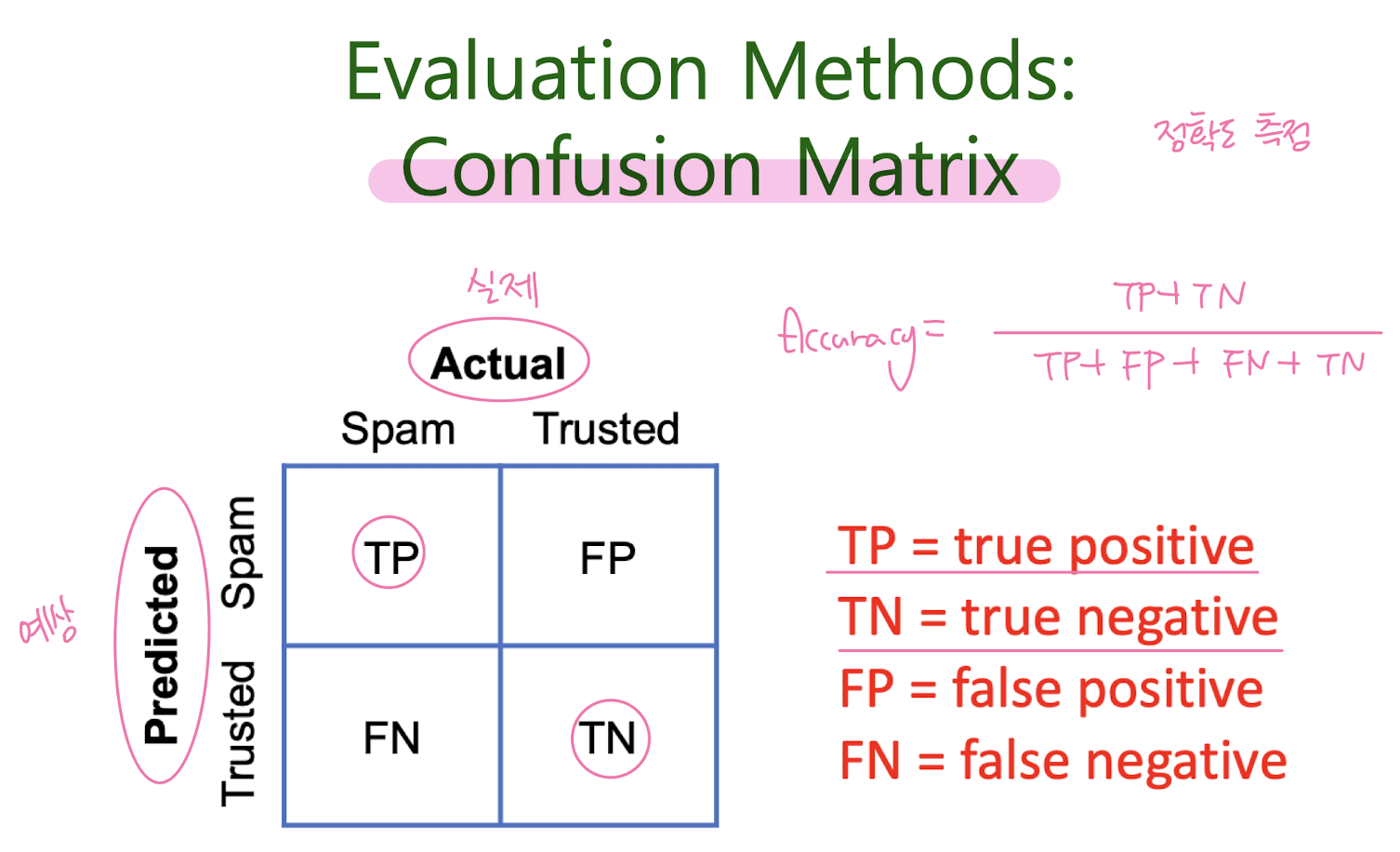
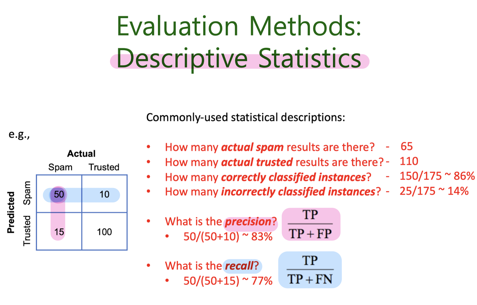
Evaluation methods
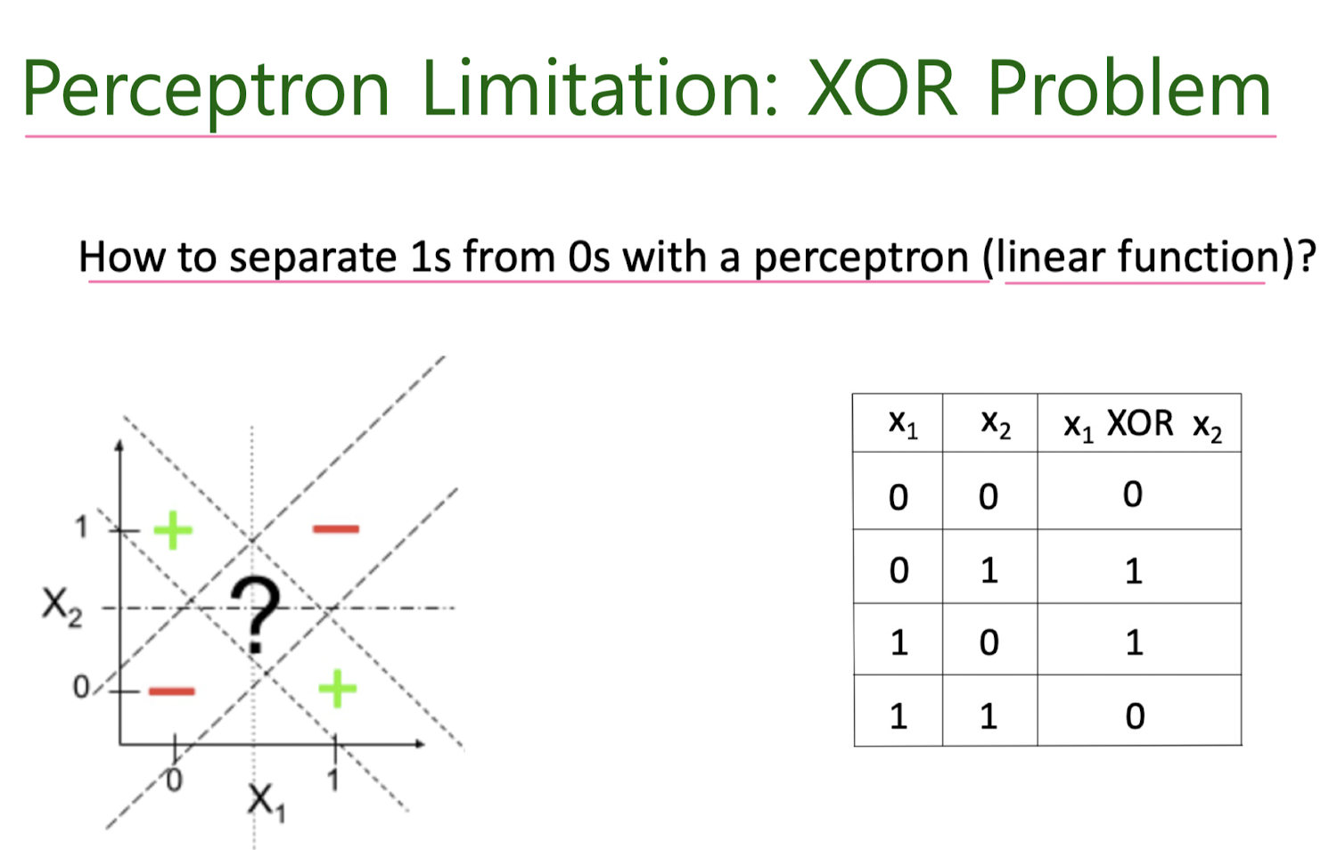
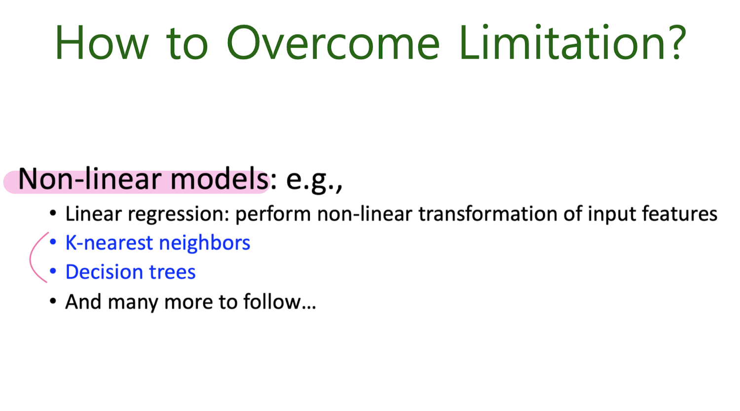
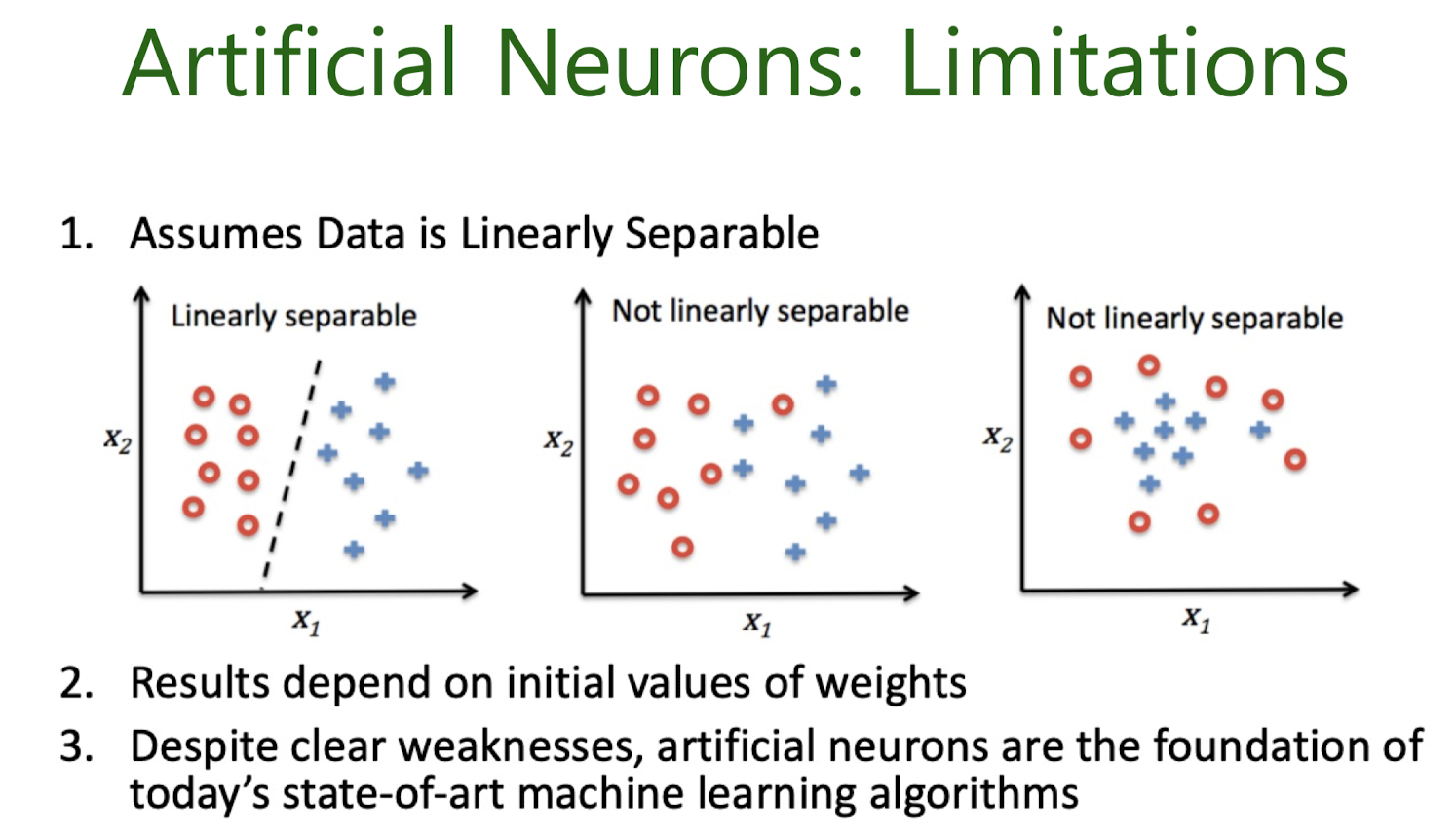
Motivation for new ML era: need non-linear models
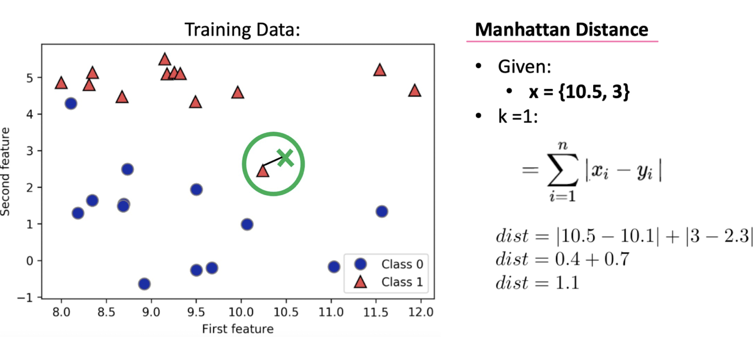
4-1. Nearest neighbor classification
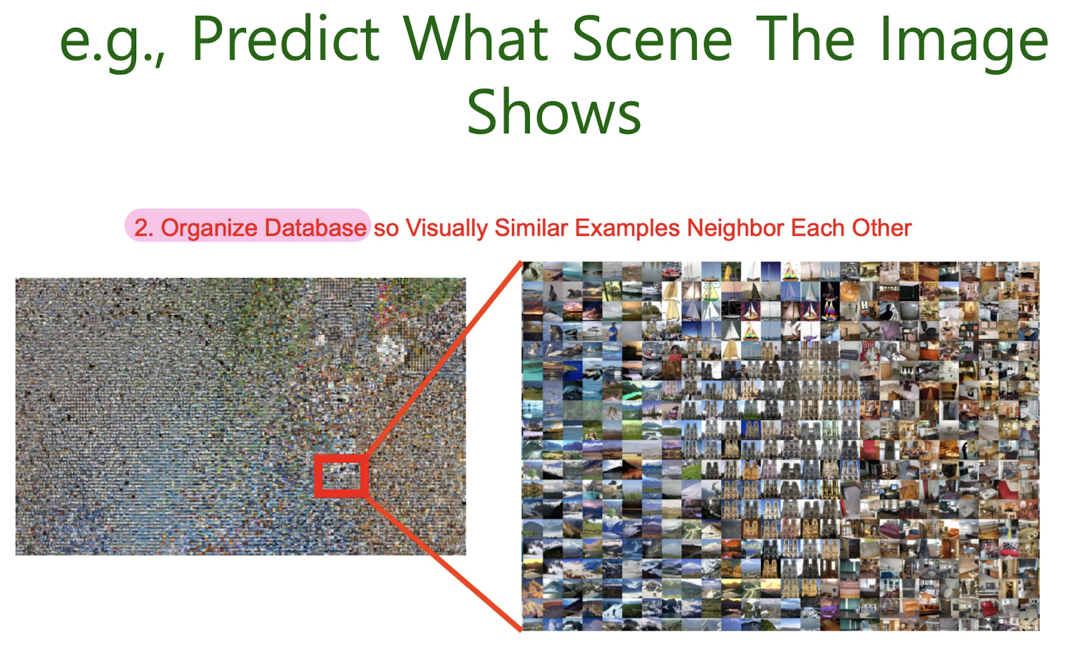
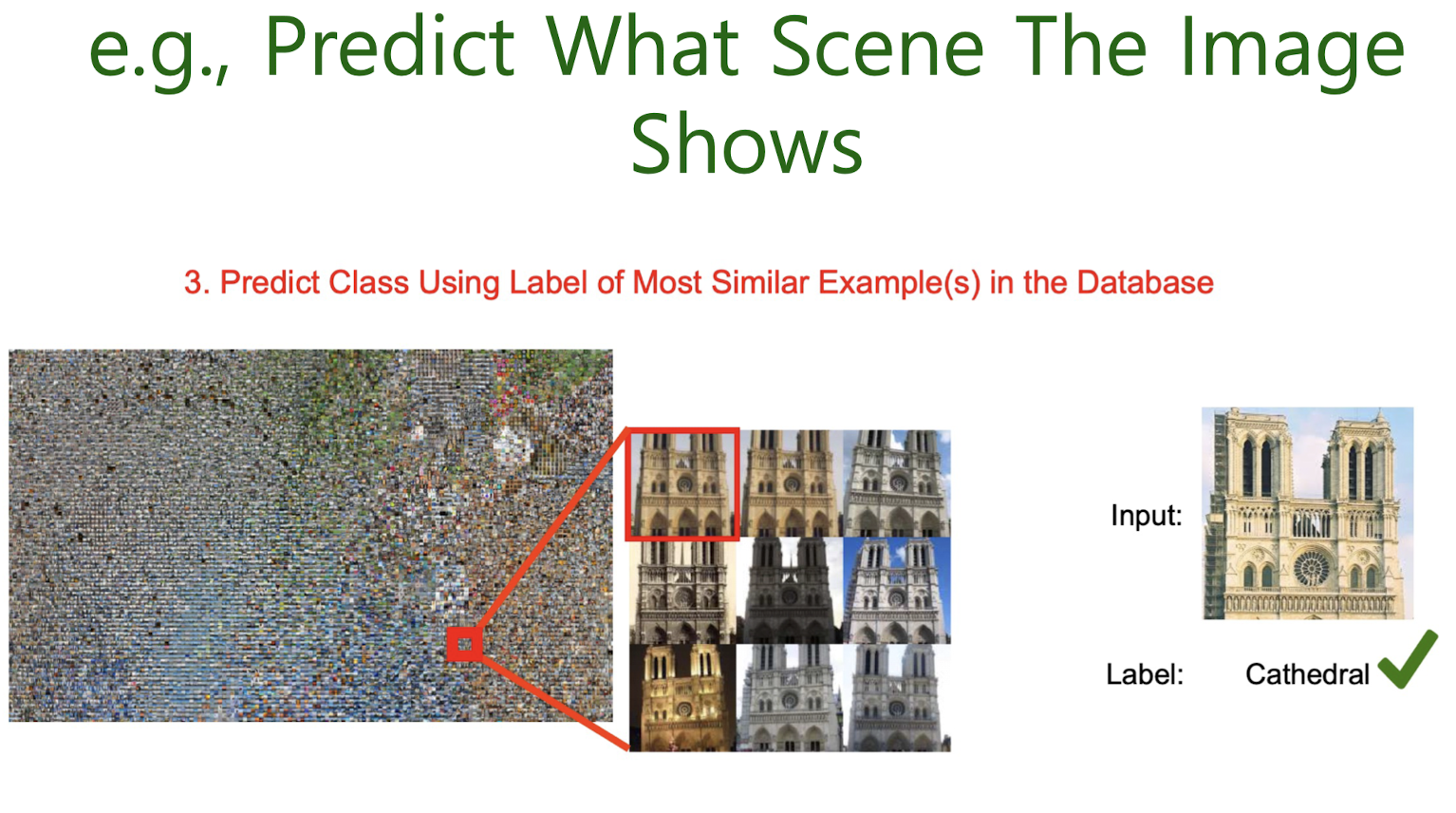
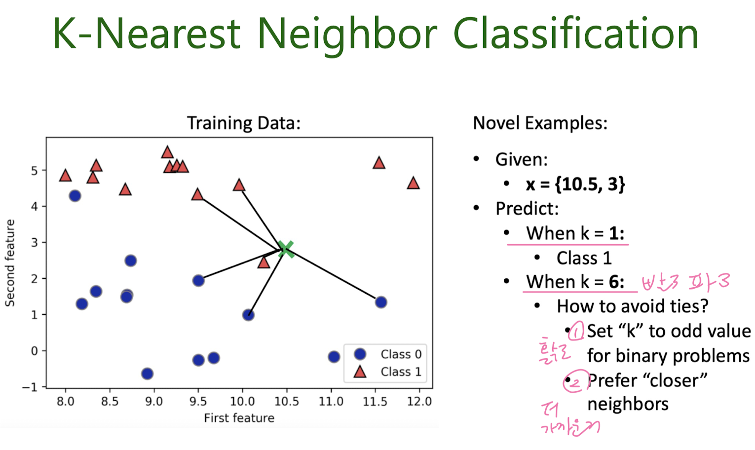
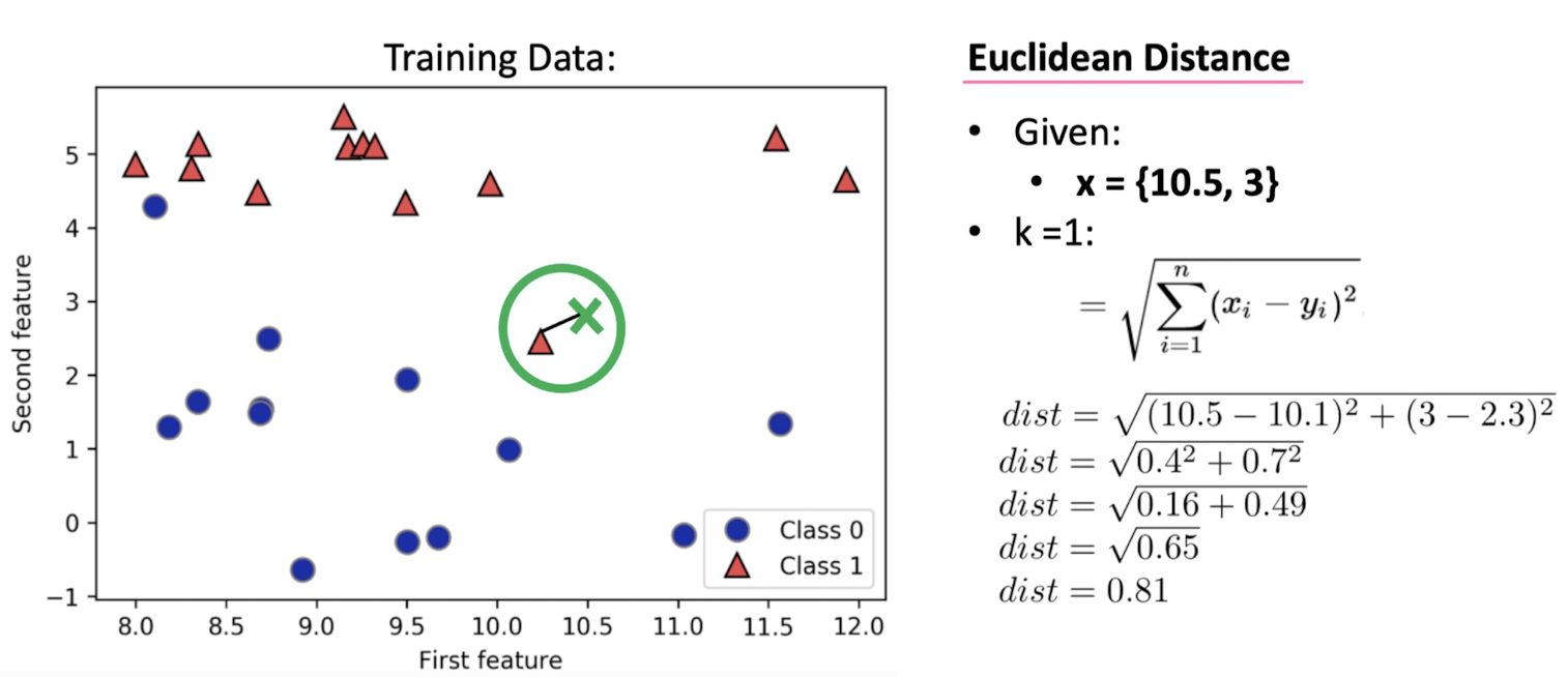
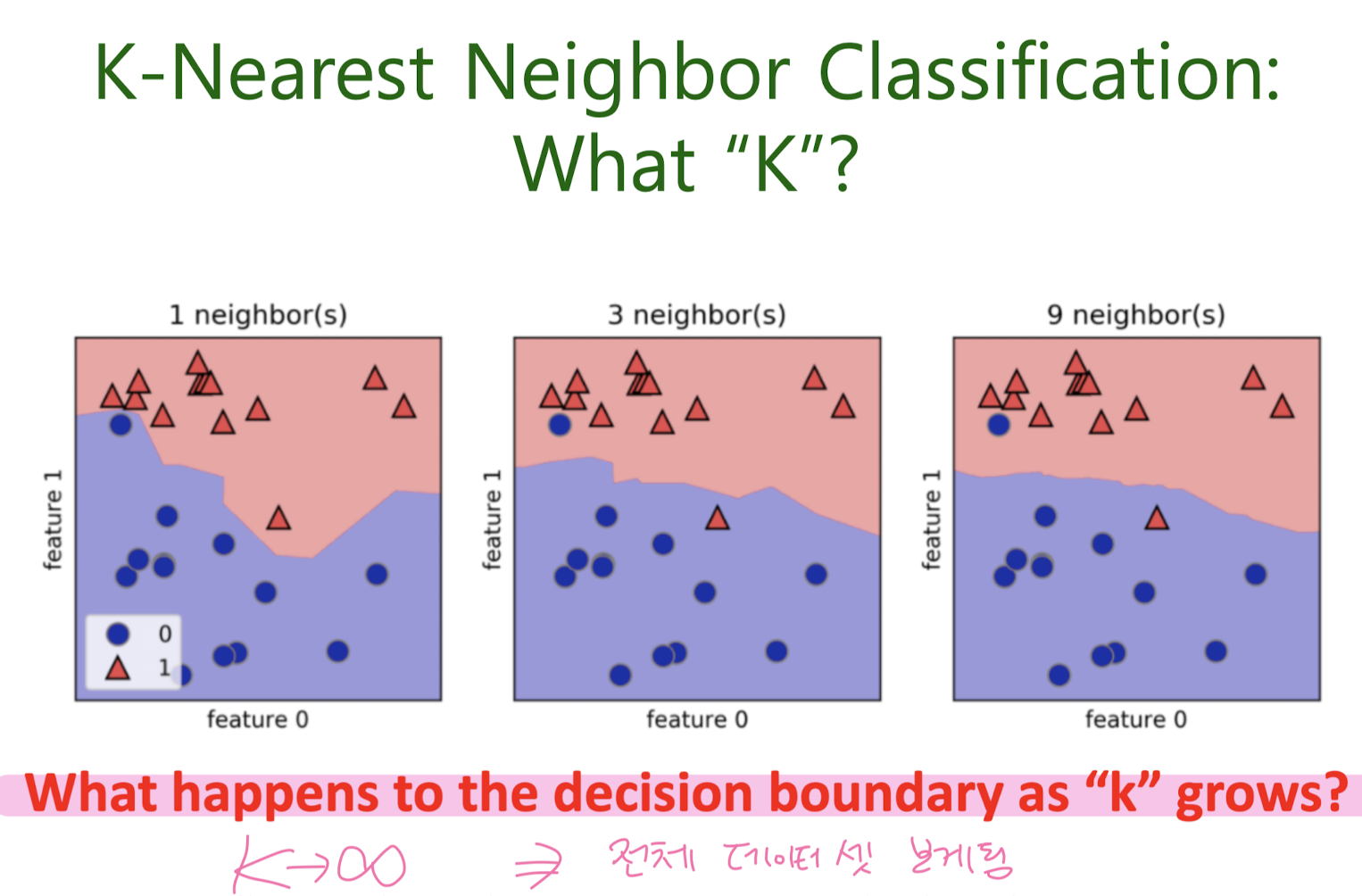
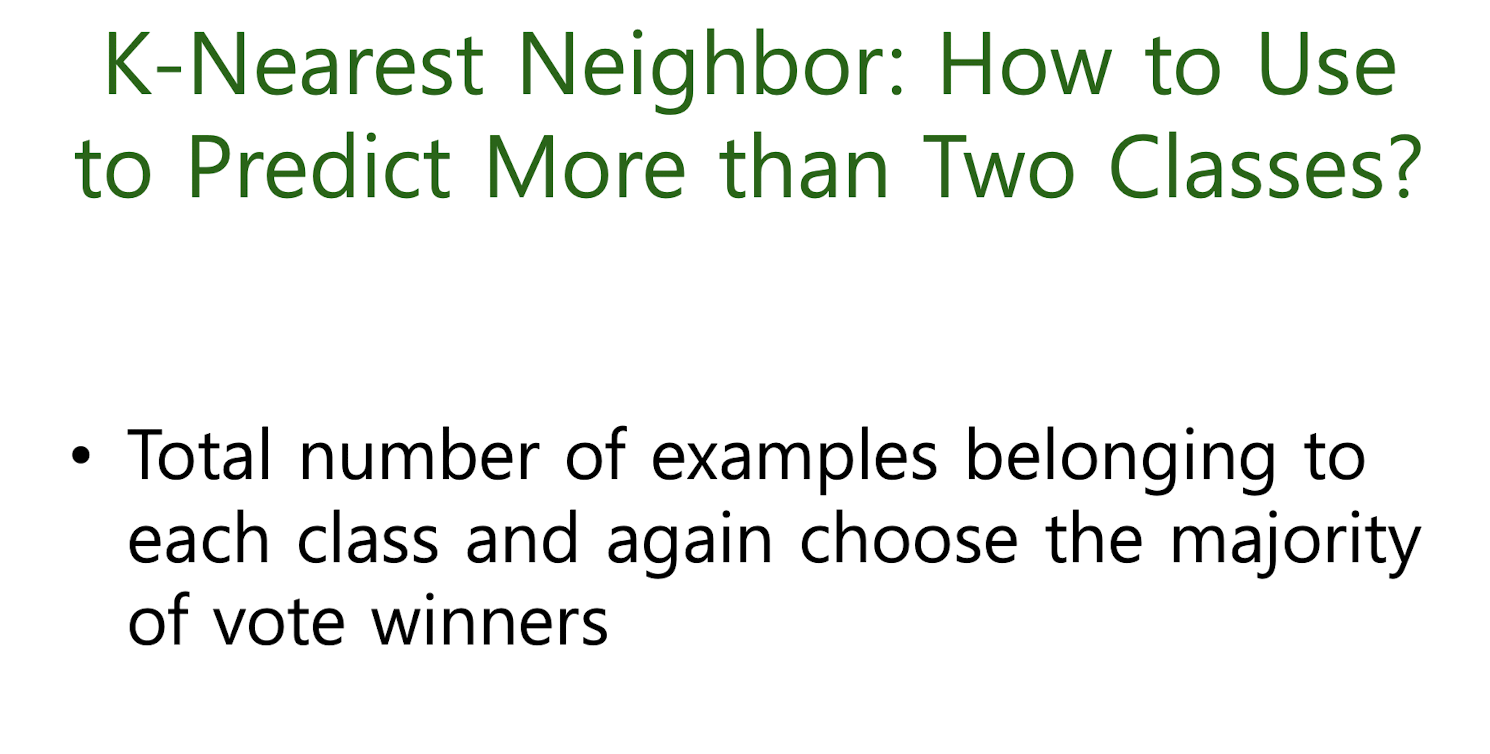
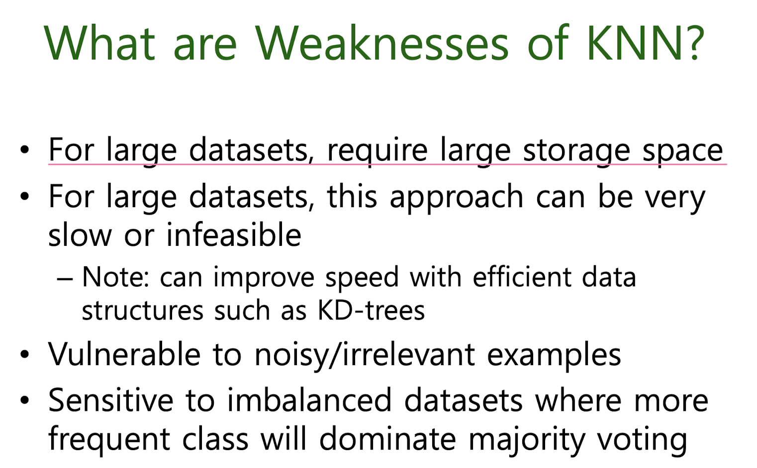
K-Nearest Neighbors
: Measuring Distance

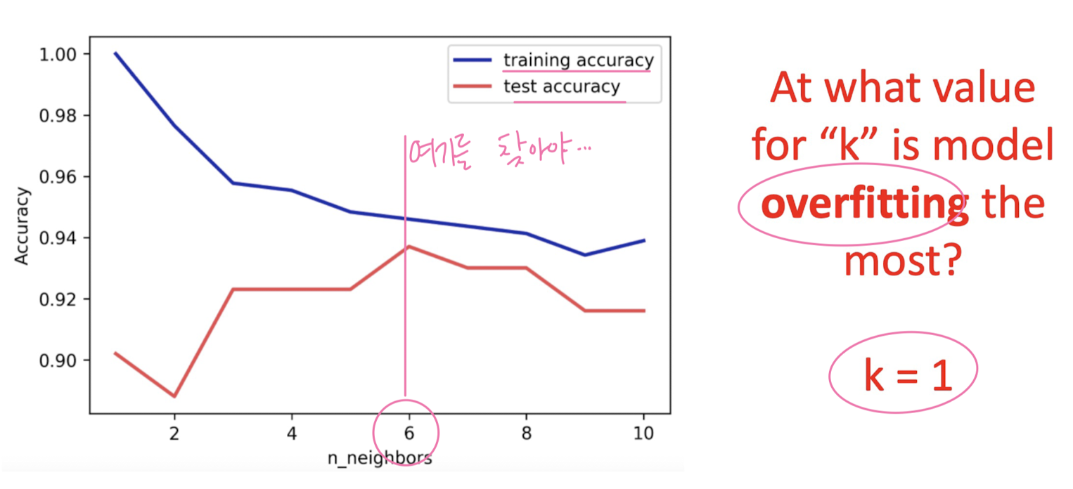
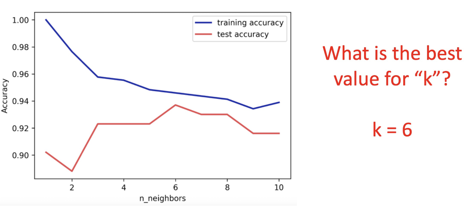
K

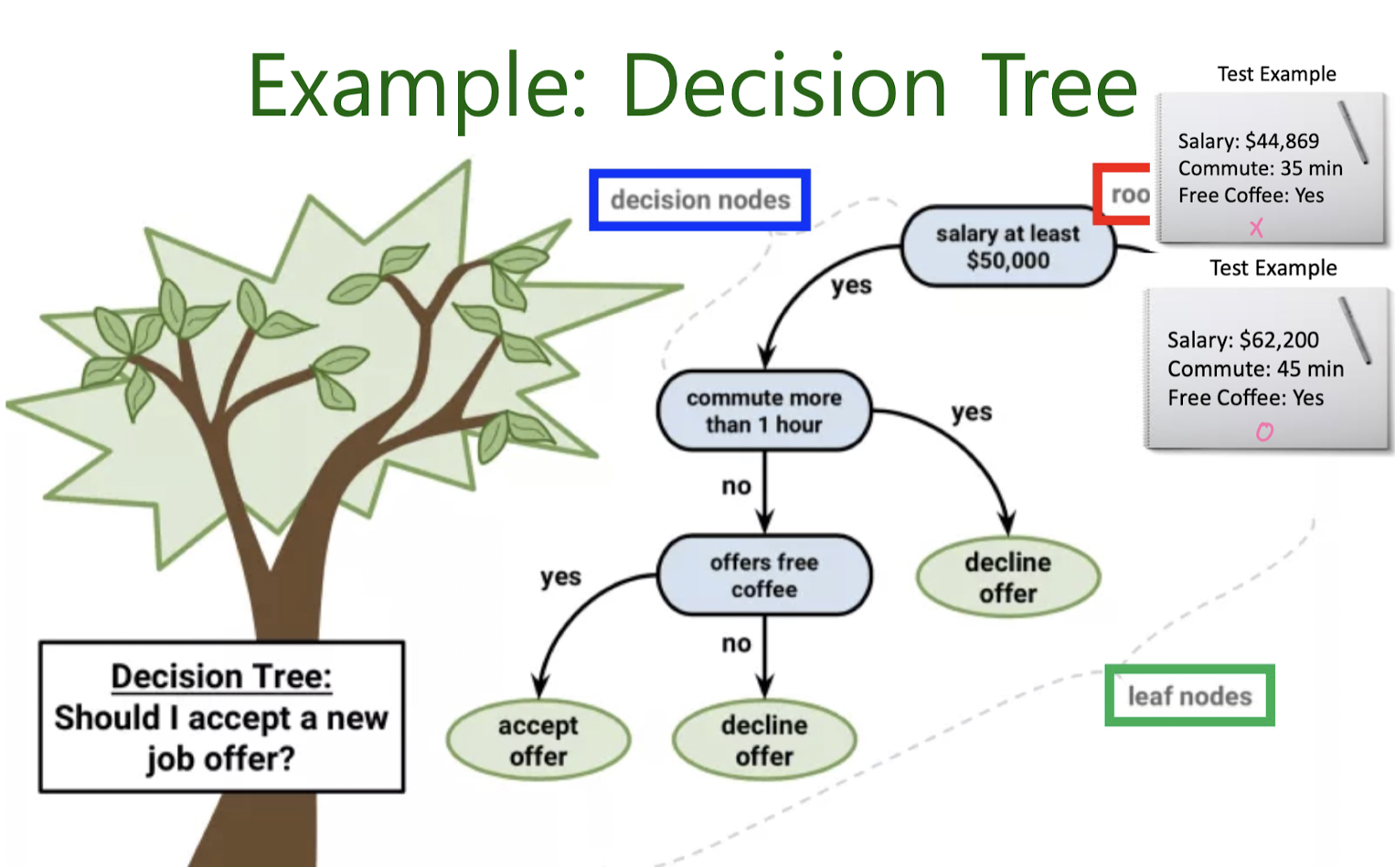
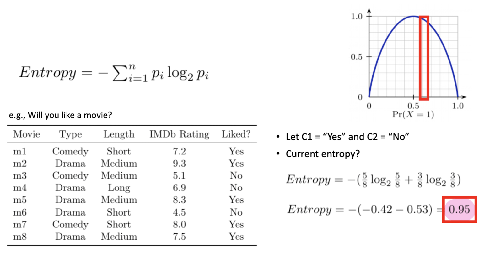
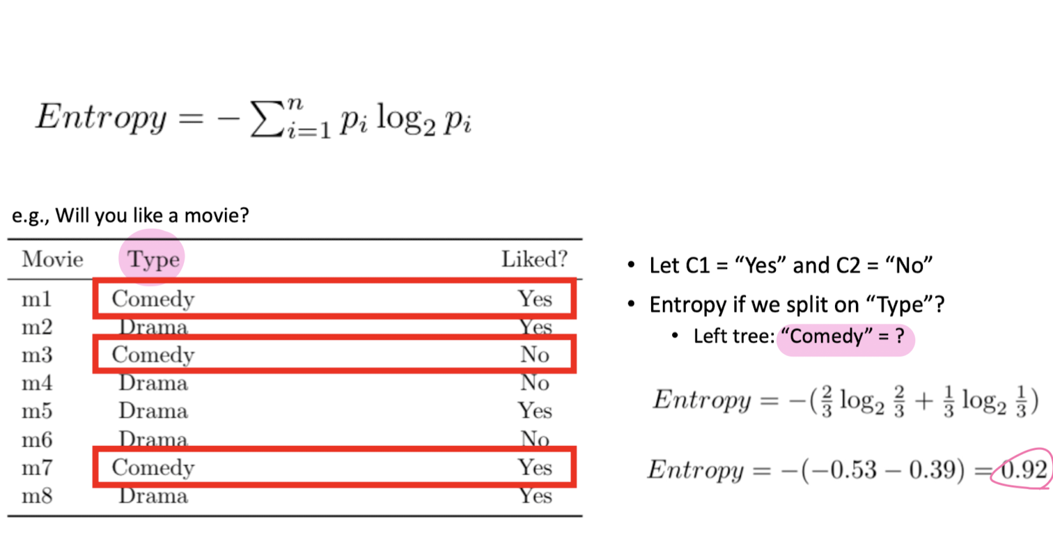
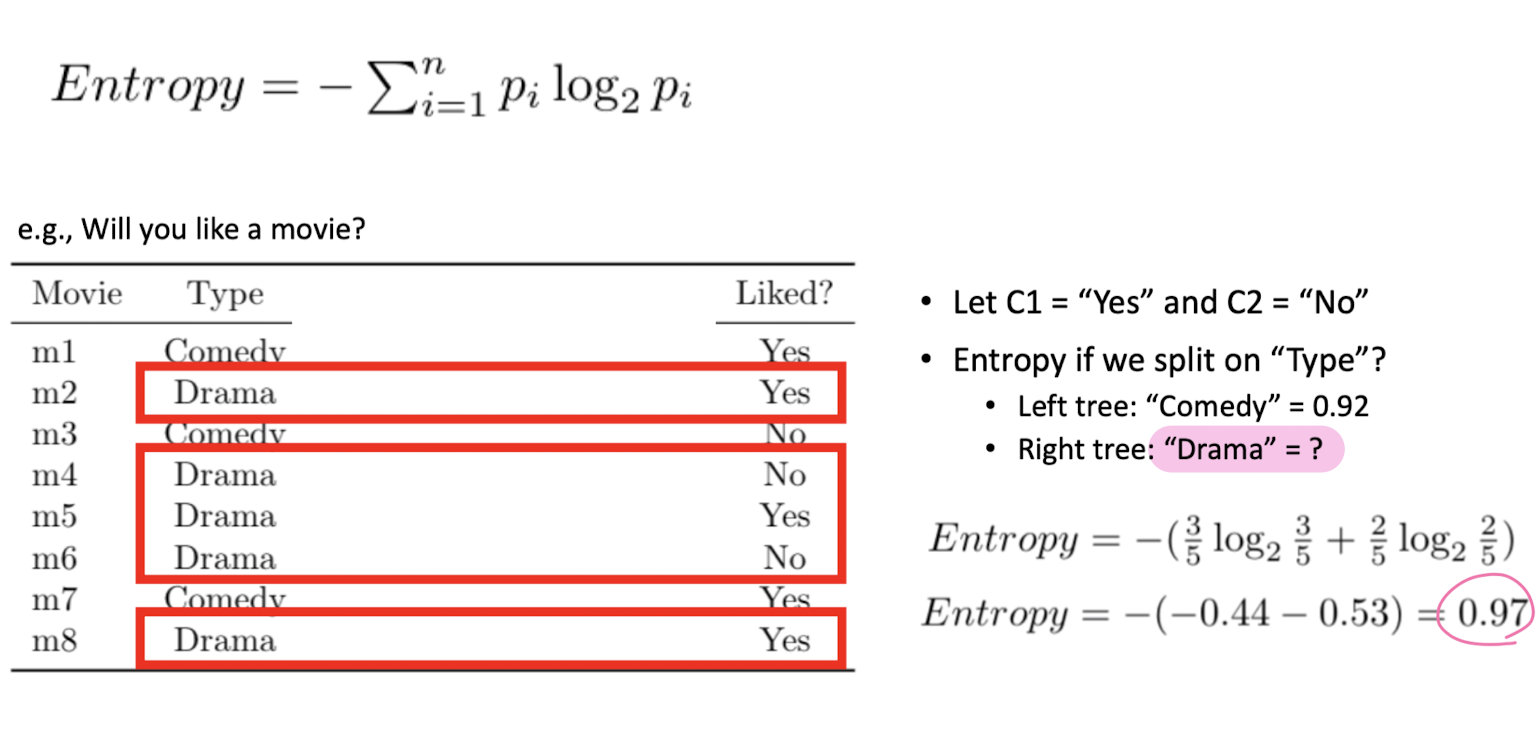
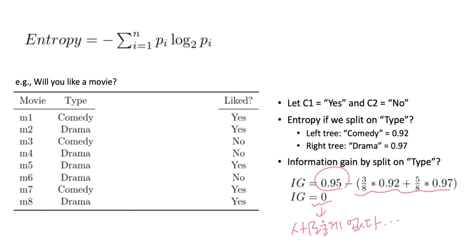
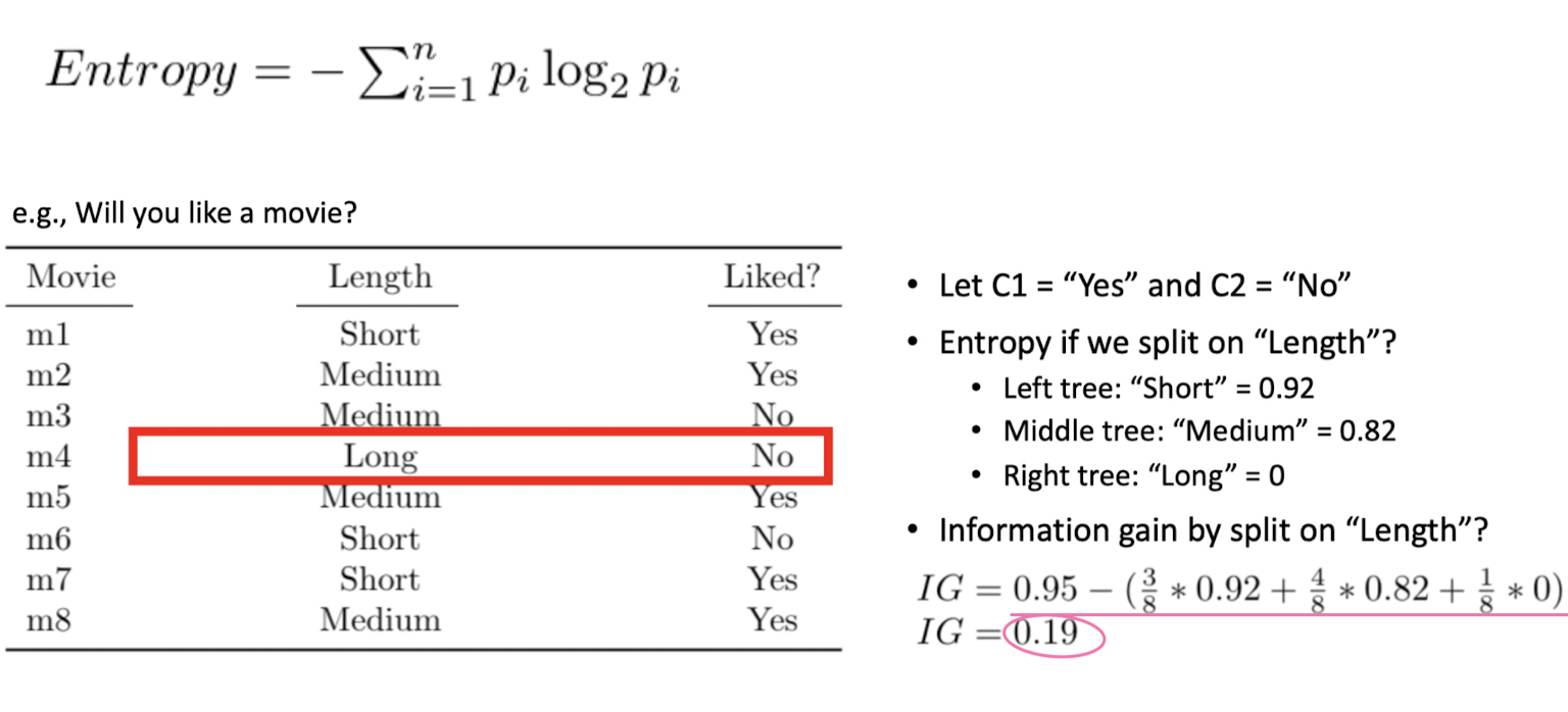
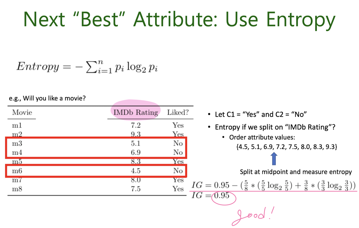
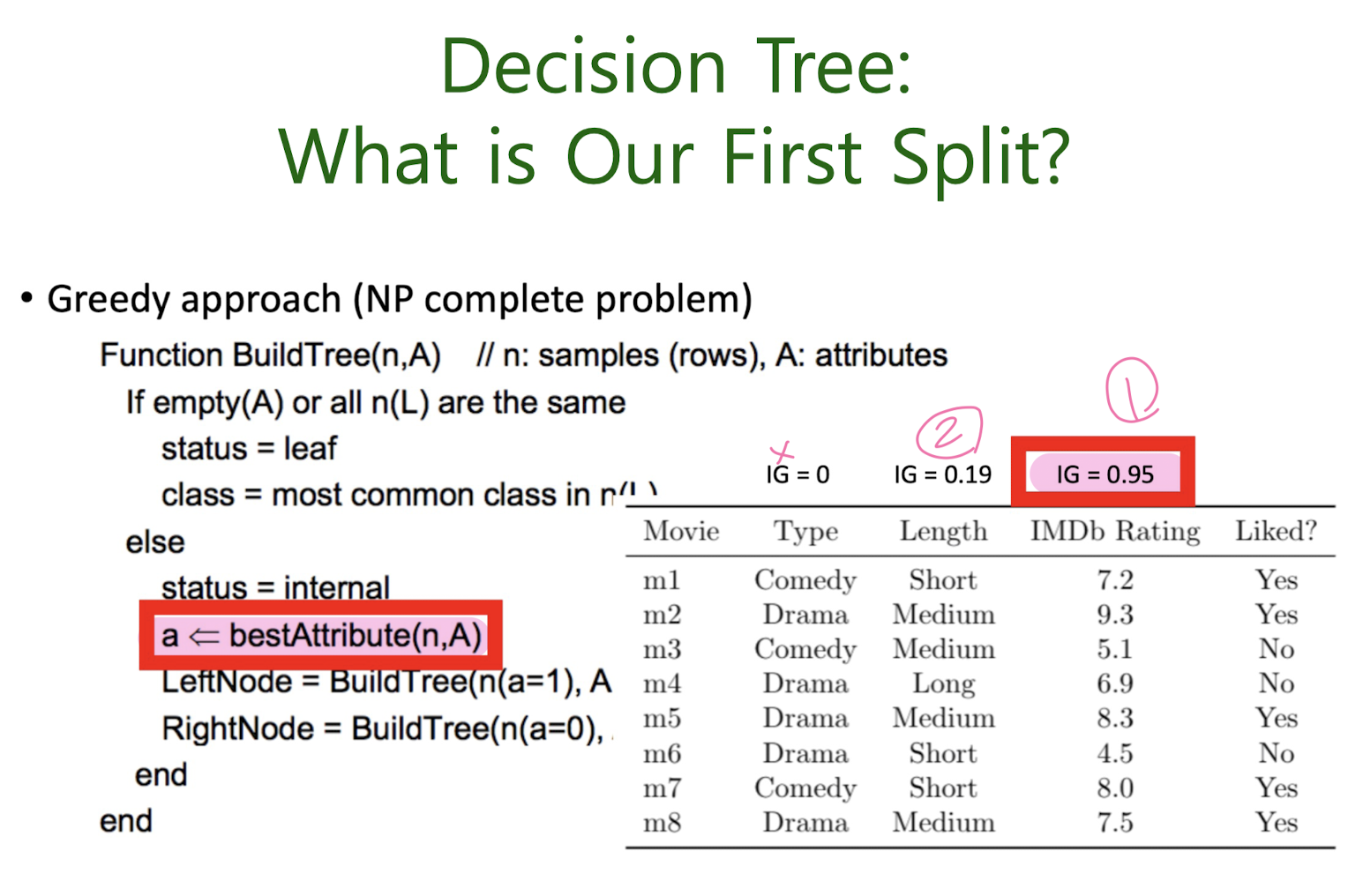
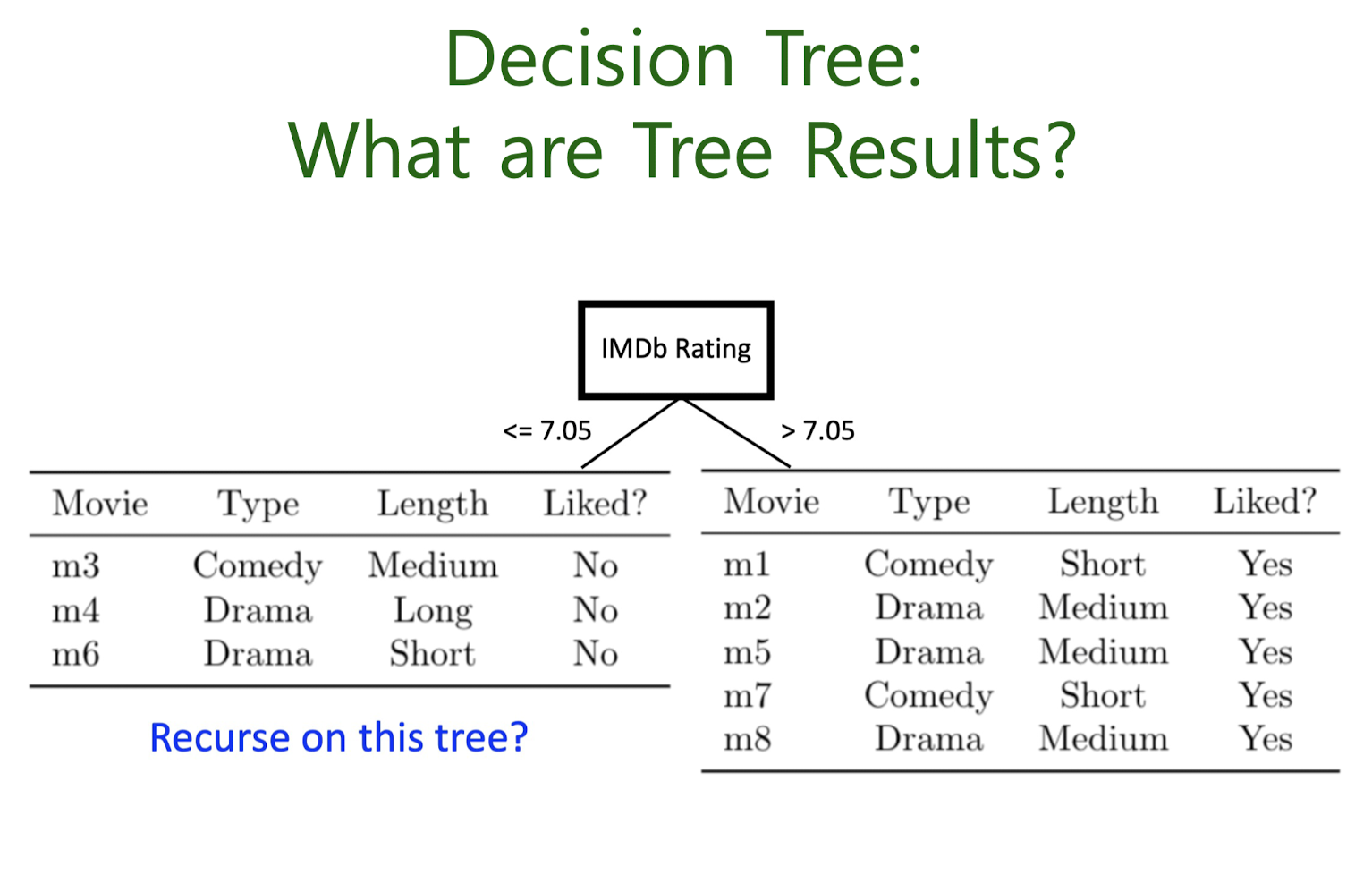
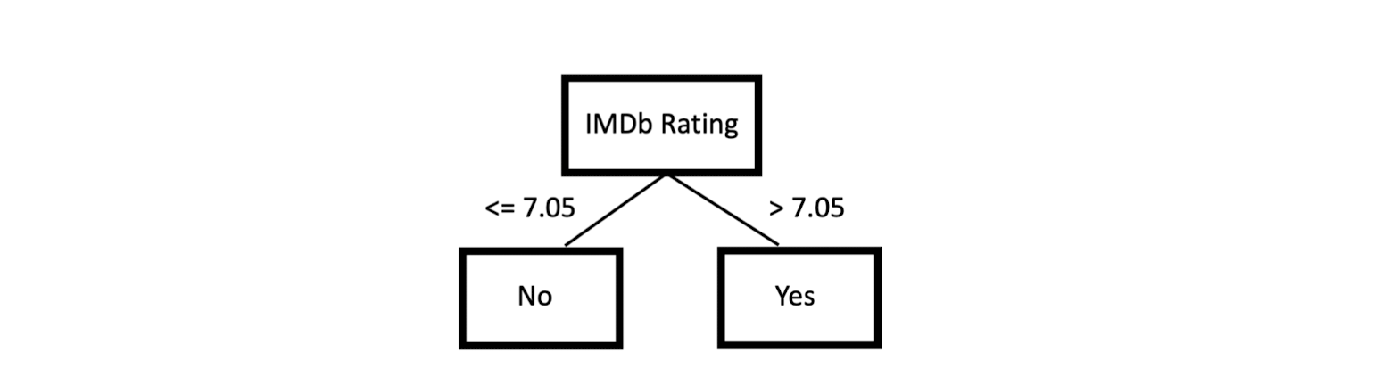
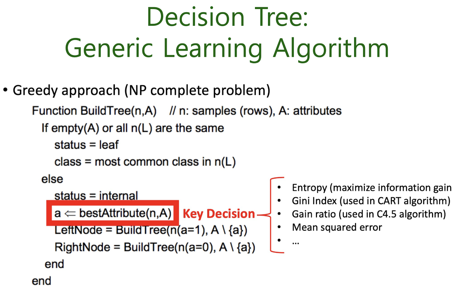
4-2. Decision tree classification
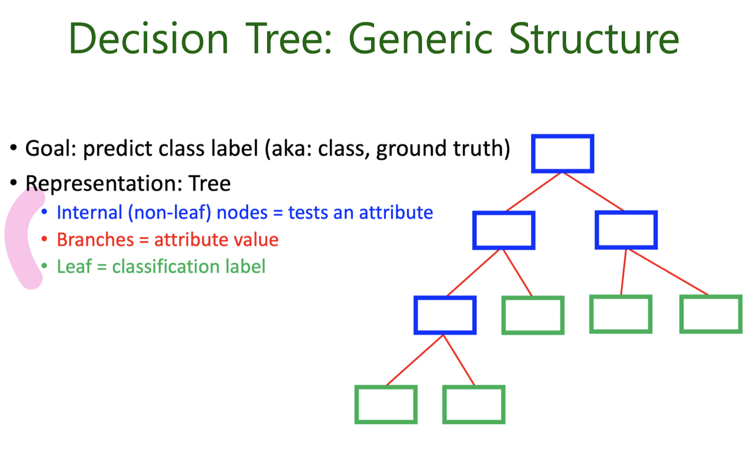
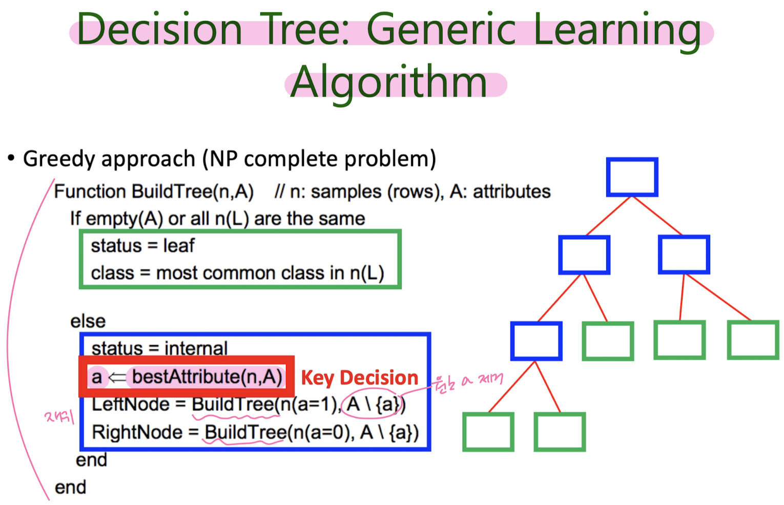
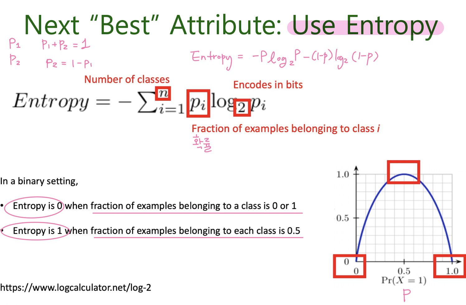
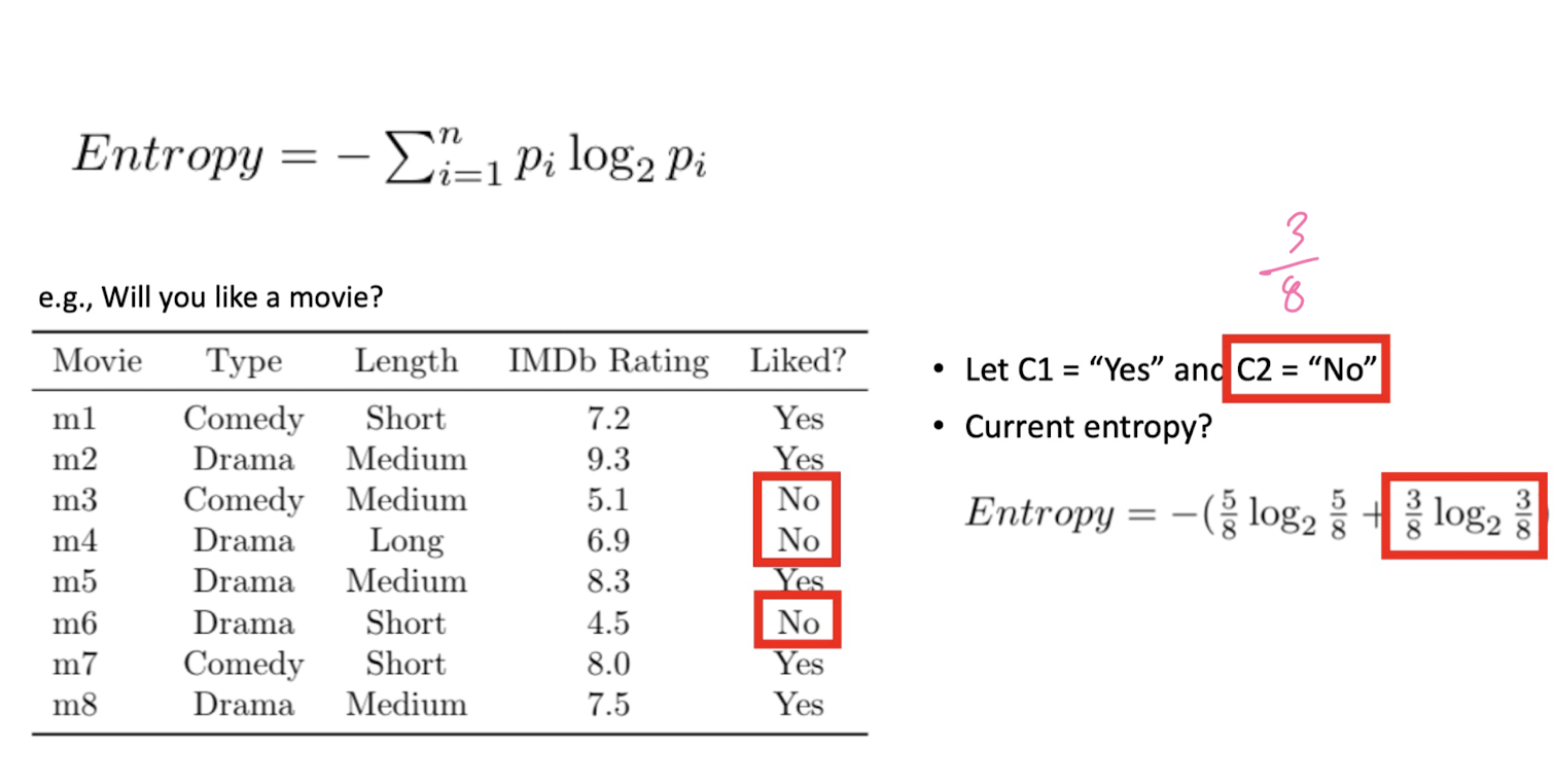
Next “Best” Attribute: Use Entropy
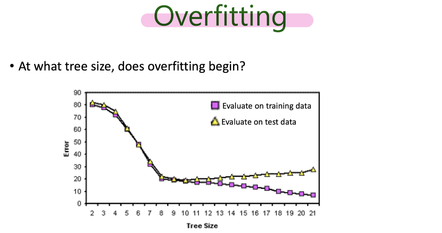
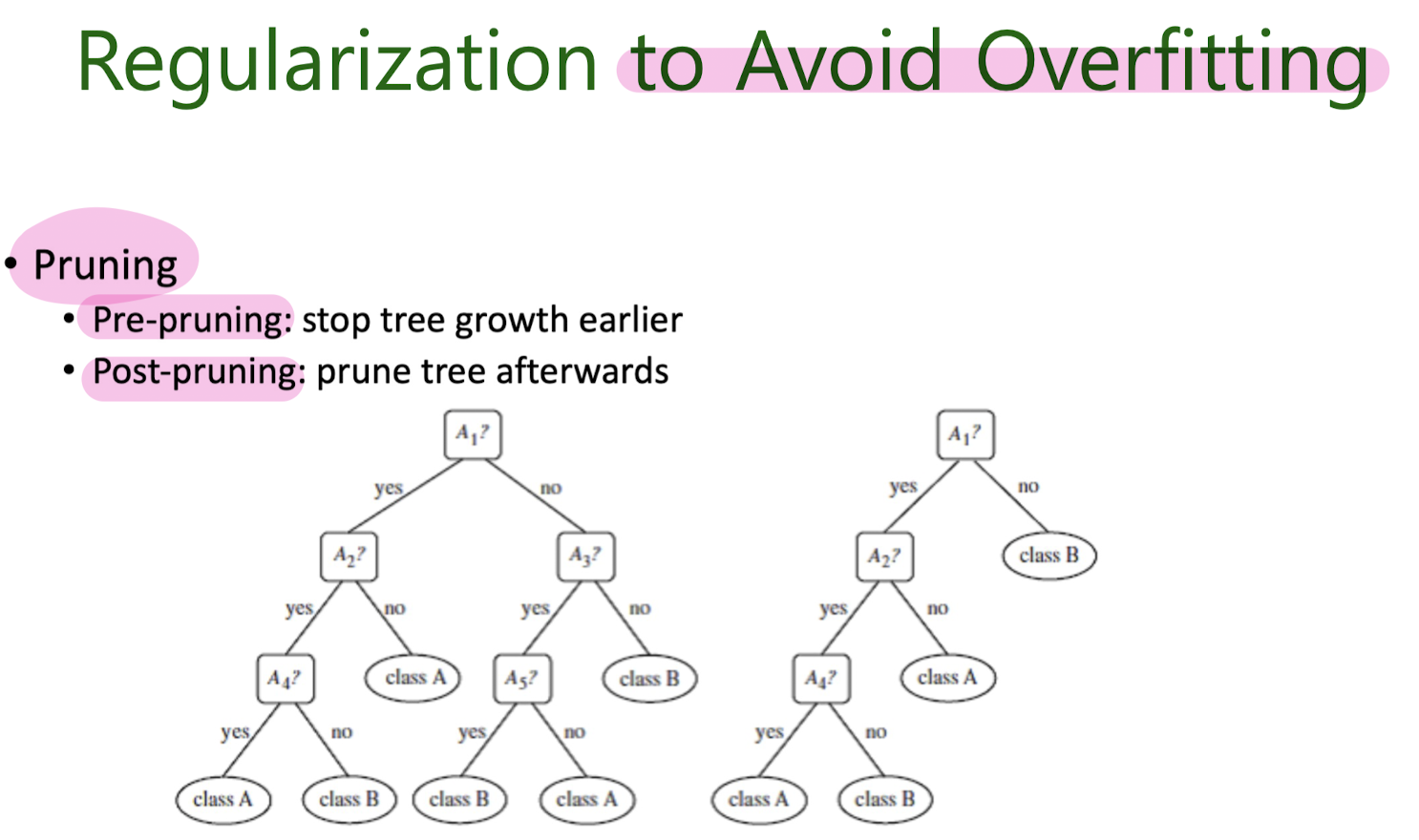
Overfitting
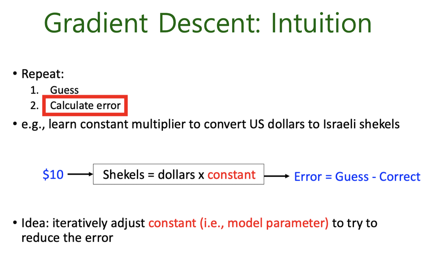
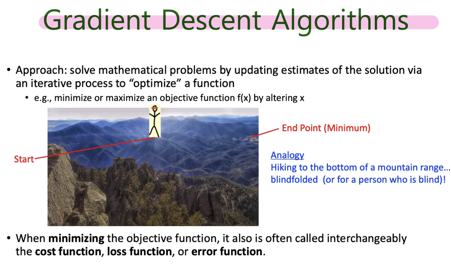
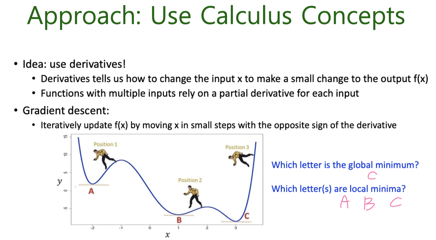
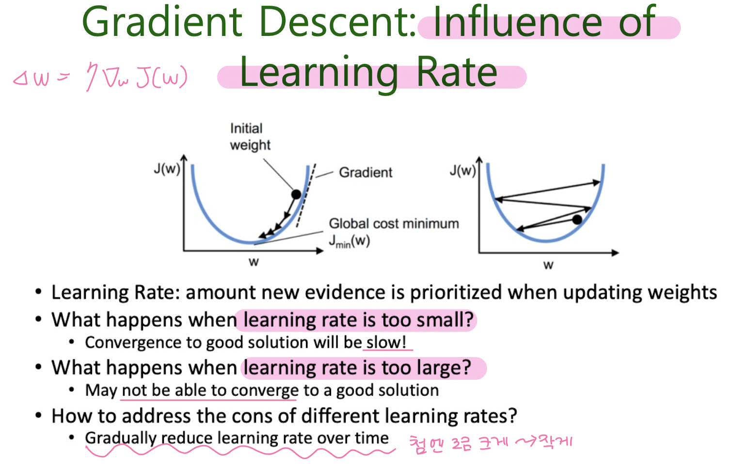
Gradient Descent
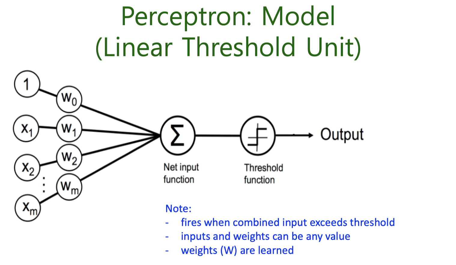
Artificial Nuurons
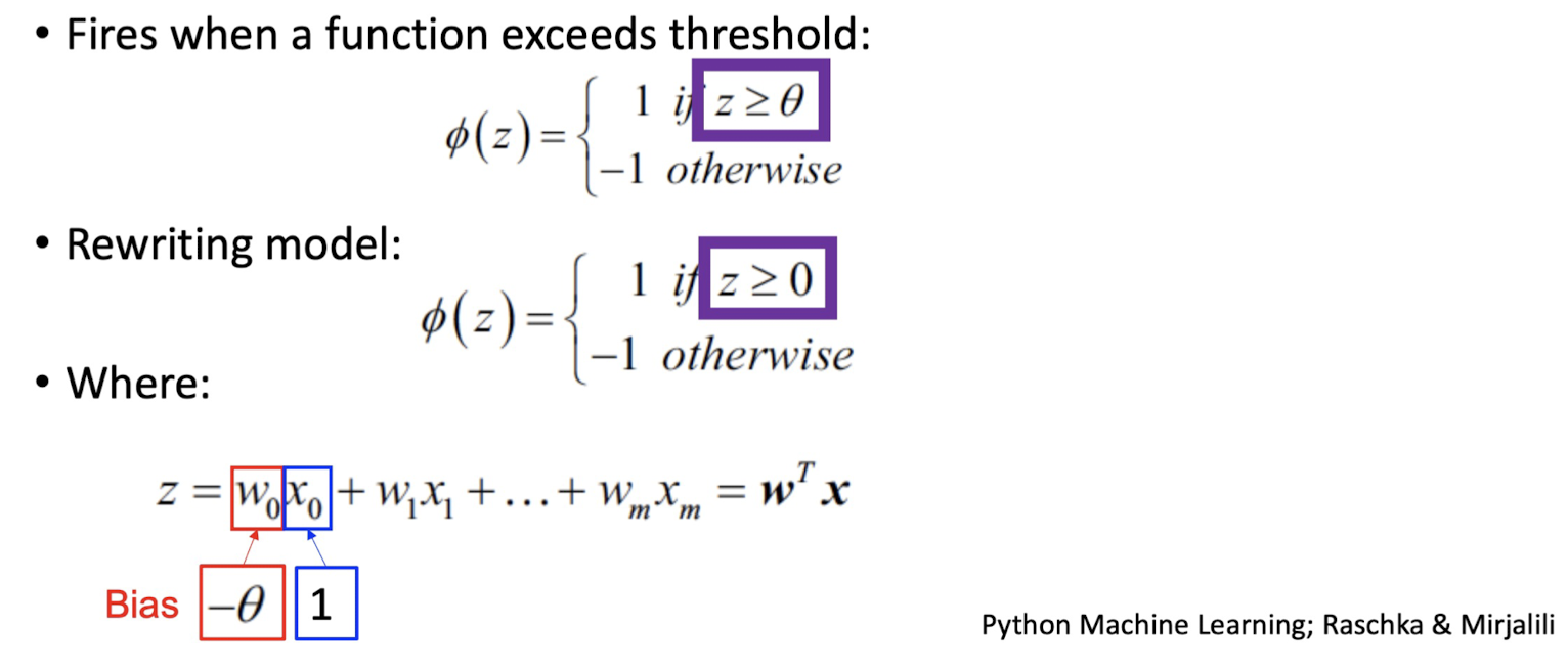
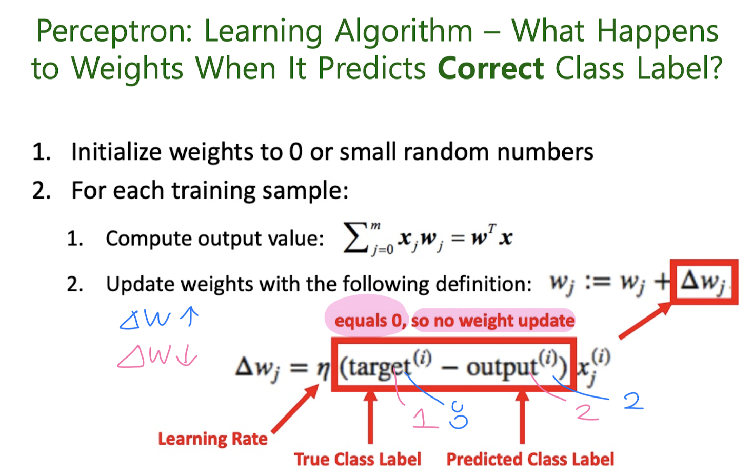
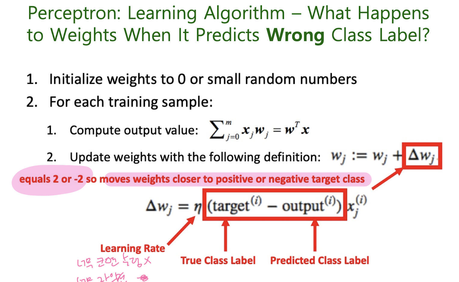
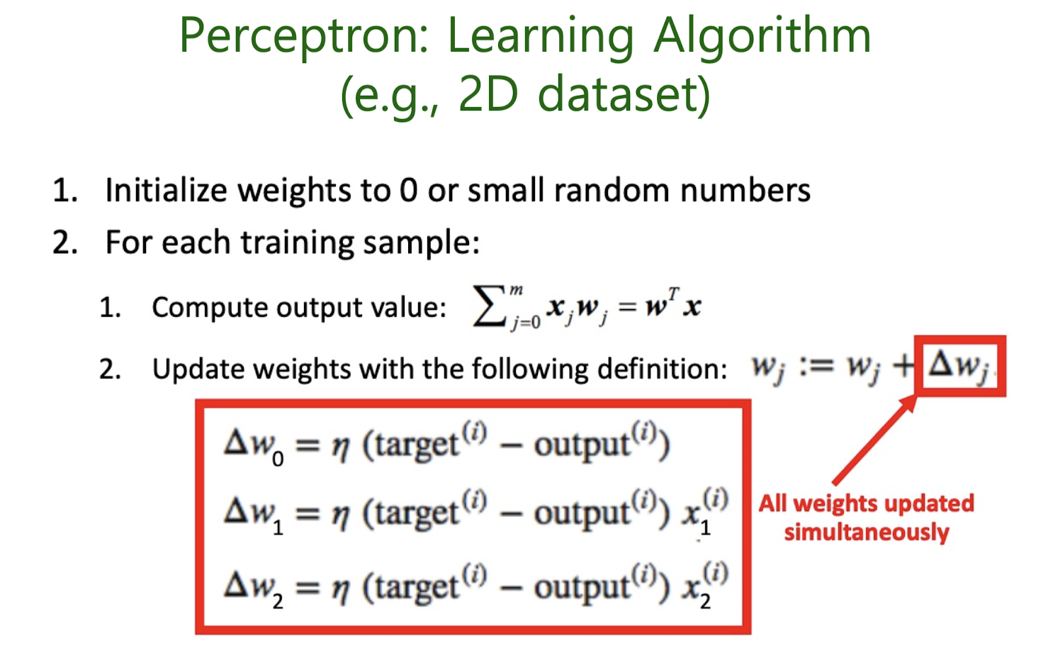
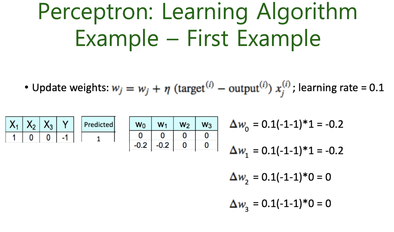
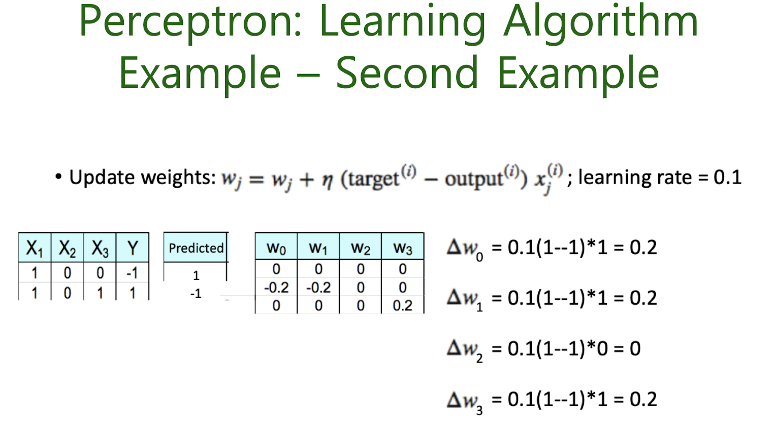
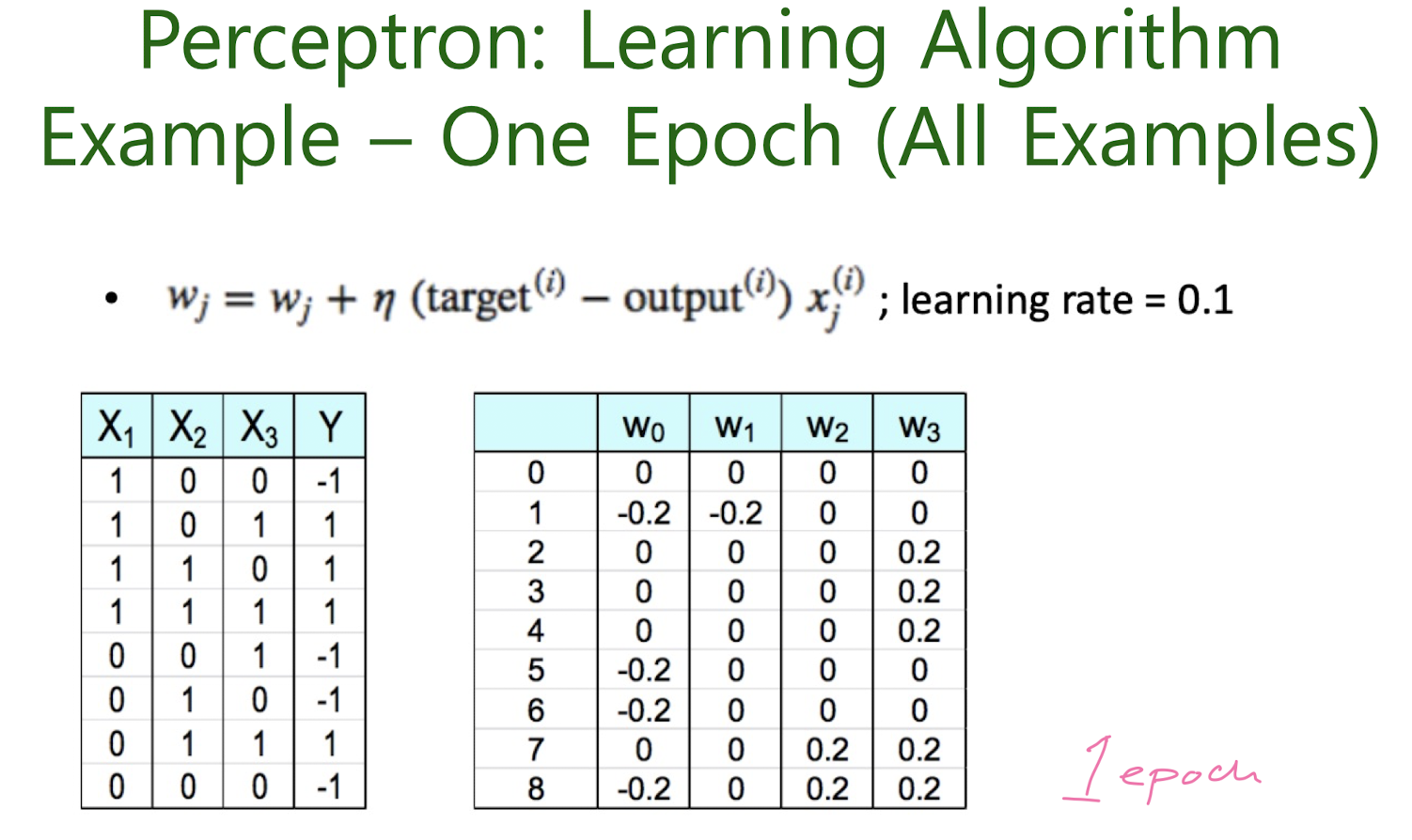
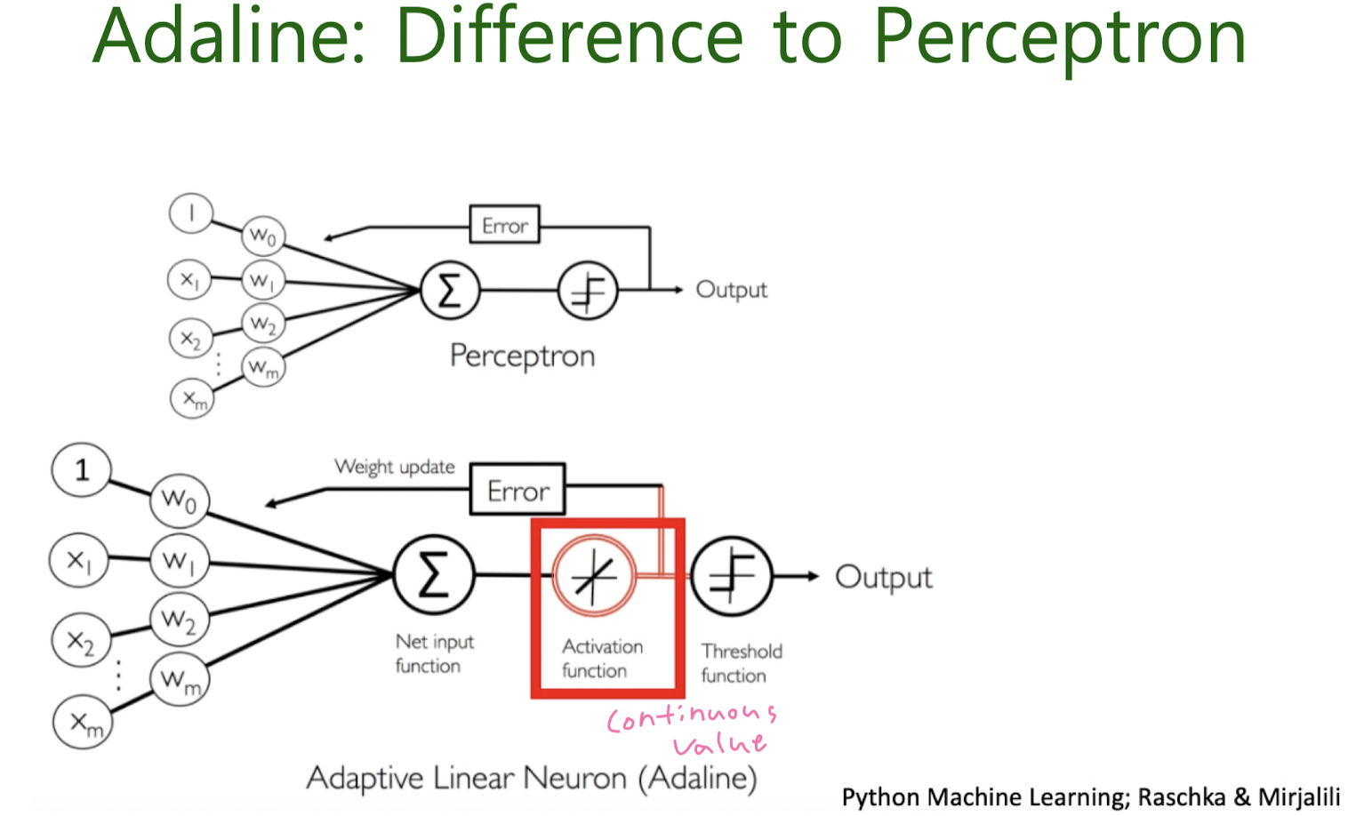
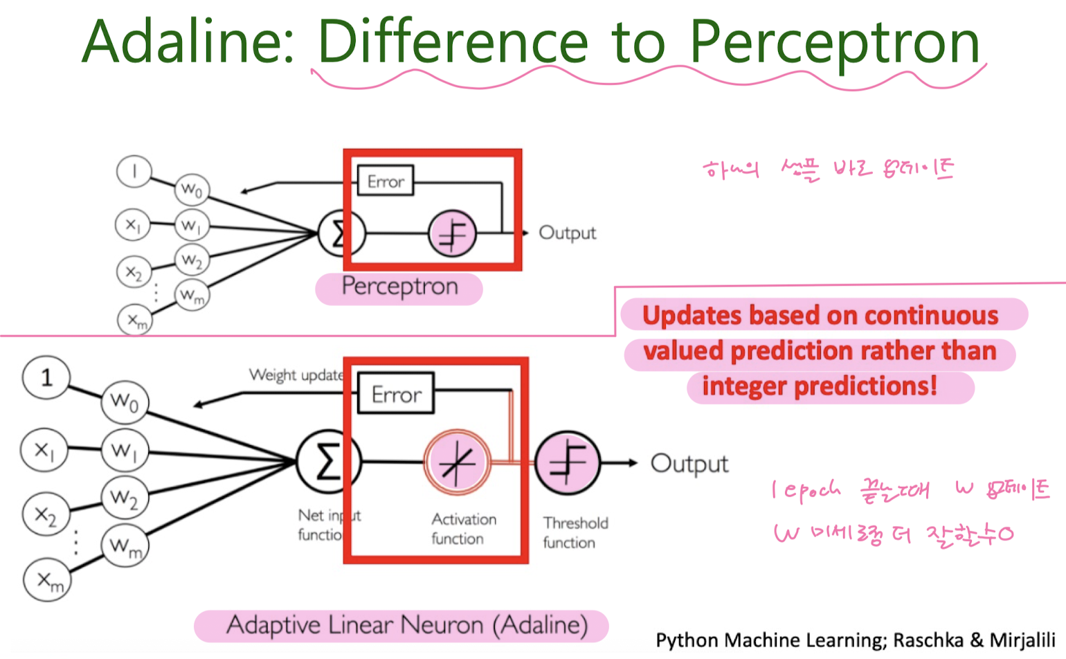
perceptron


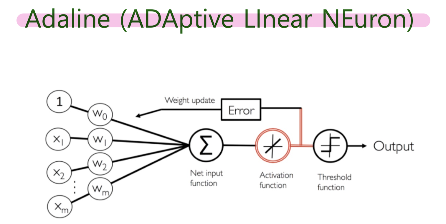
Adaline (ADAptive LInear NEuron)
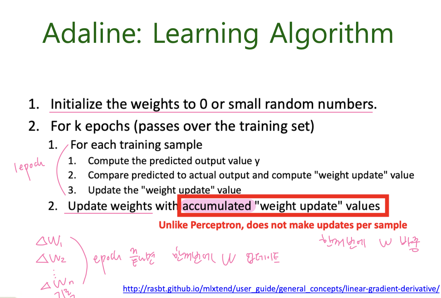
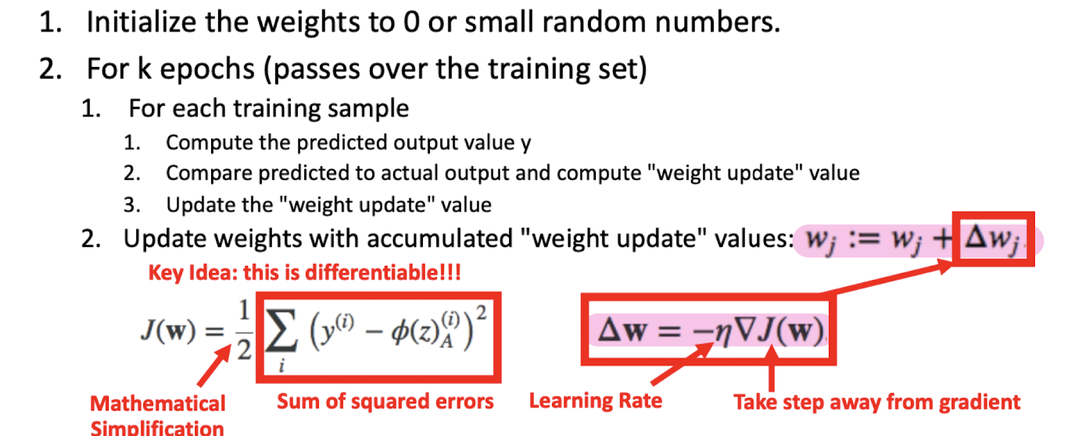

Gradient Descent
Batch Gradient Descent (BGD)

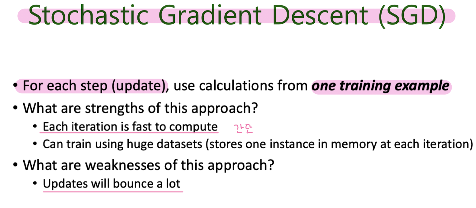
Stochastic Gradient Descent (SGD)
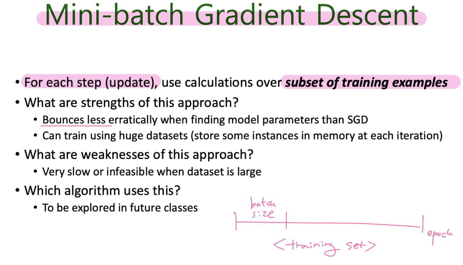
Mini-batch Gradient Descent
5. Classification: Naive Bayes, SVM
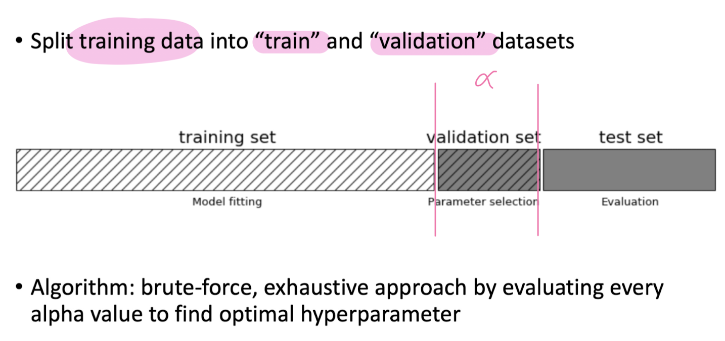
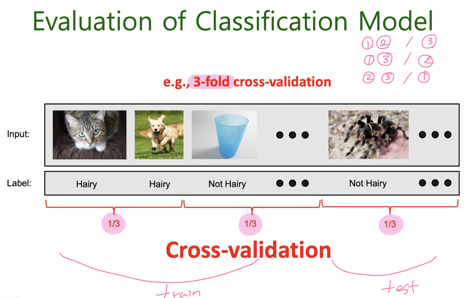
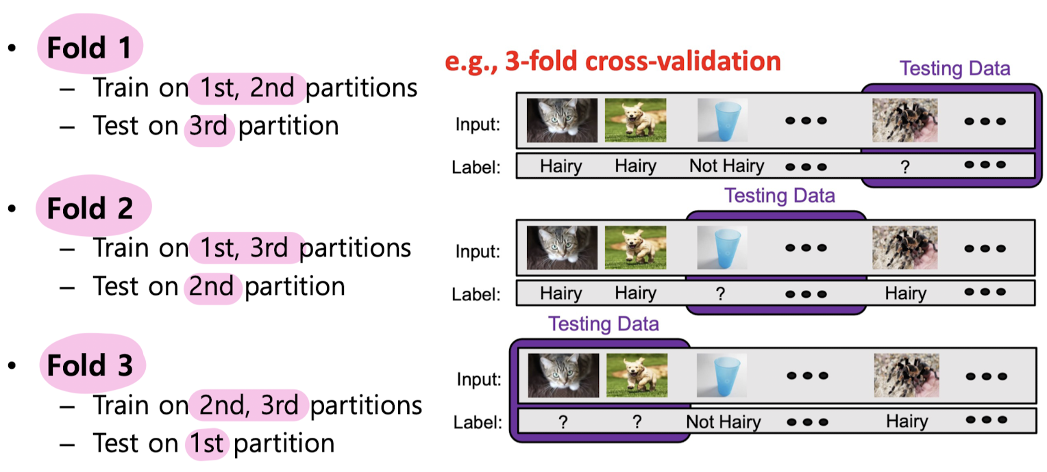
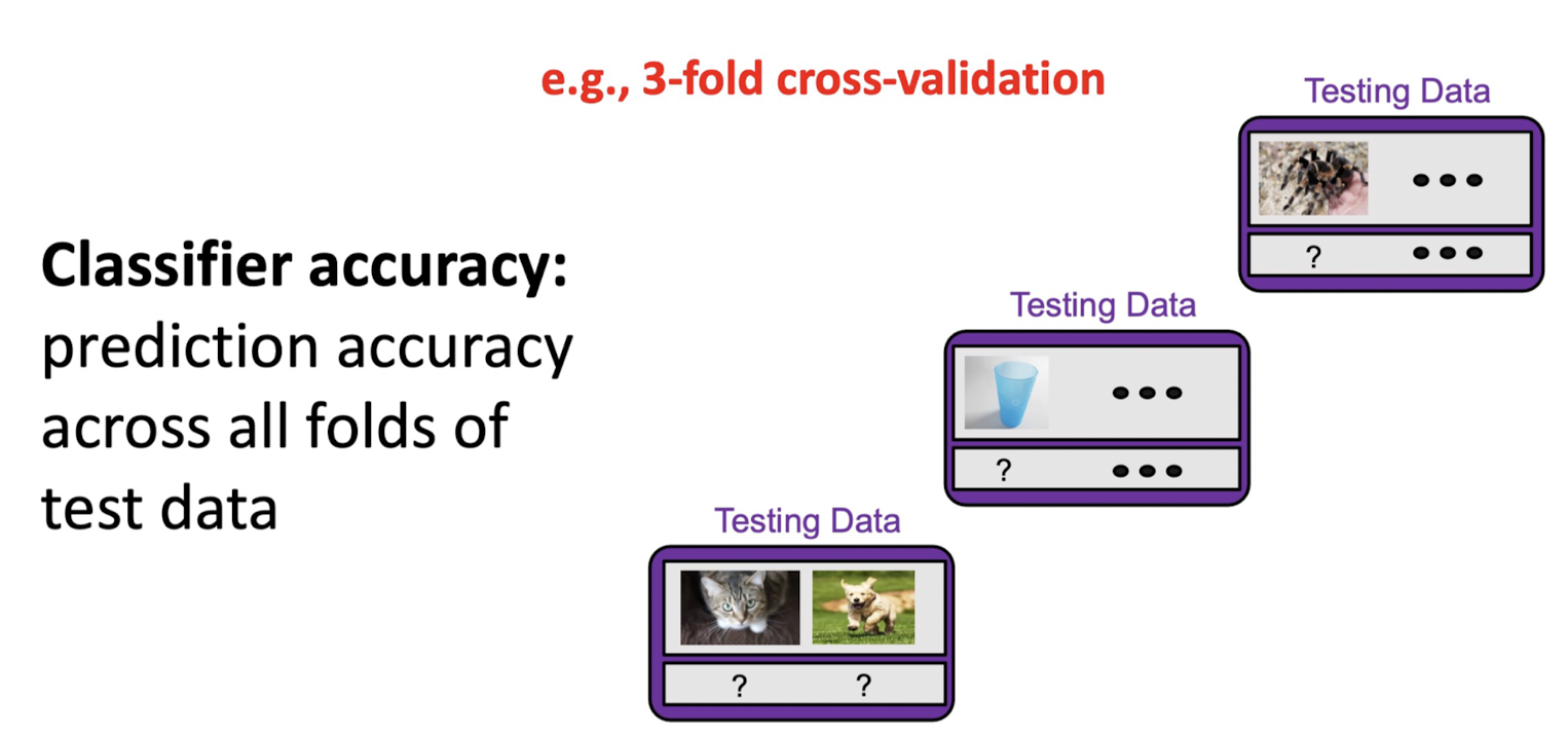
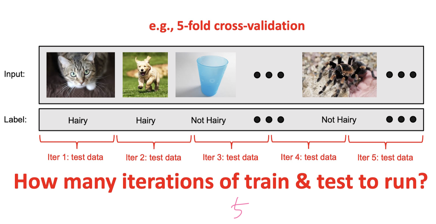
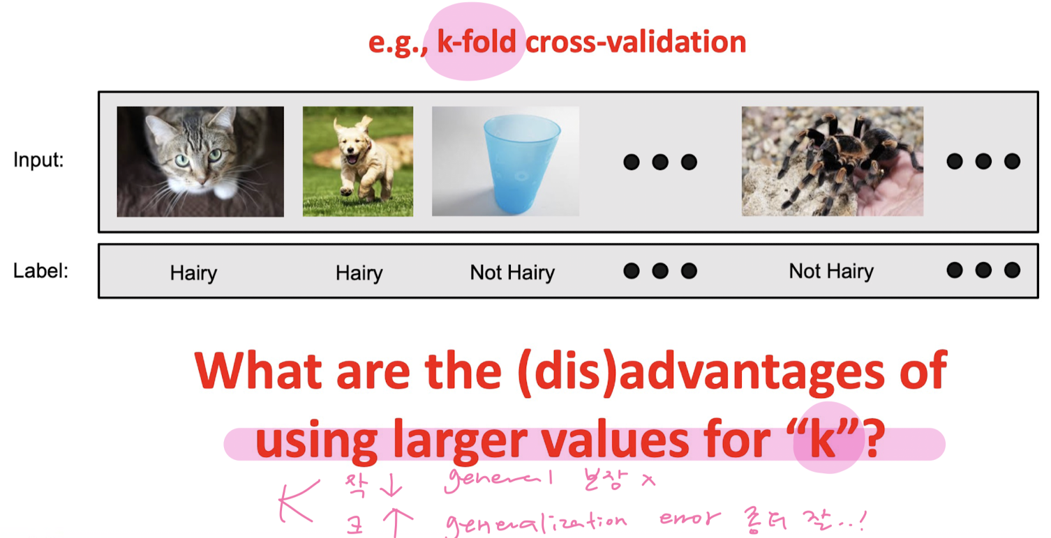
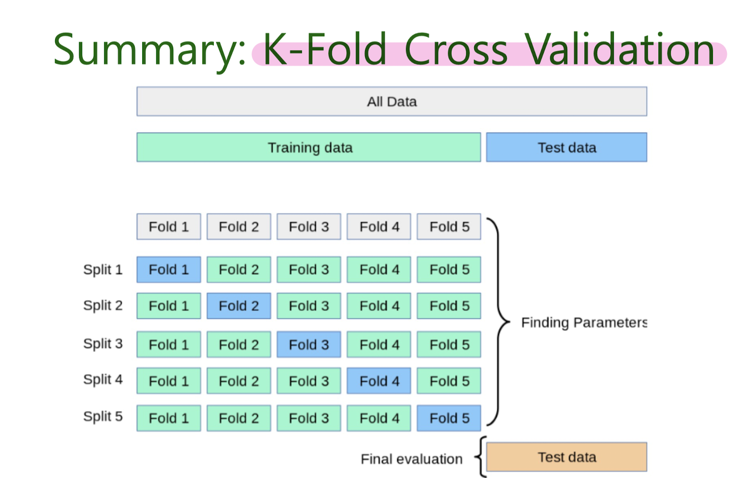
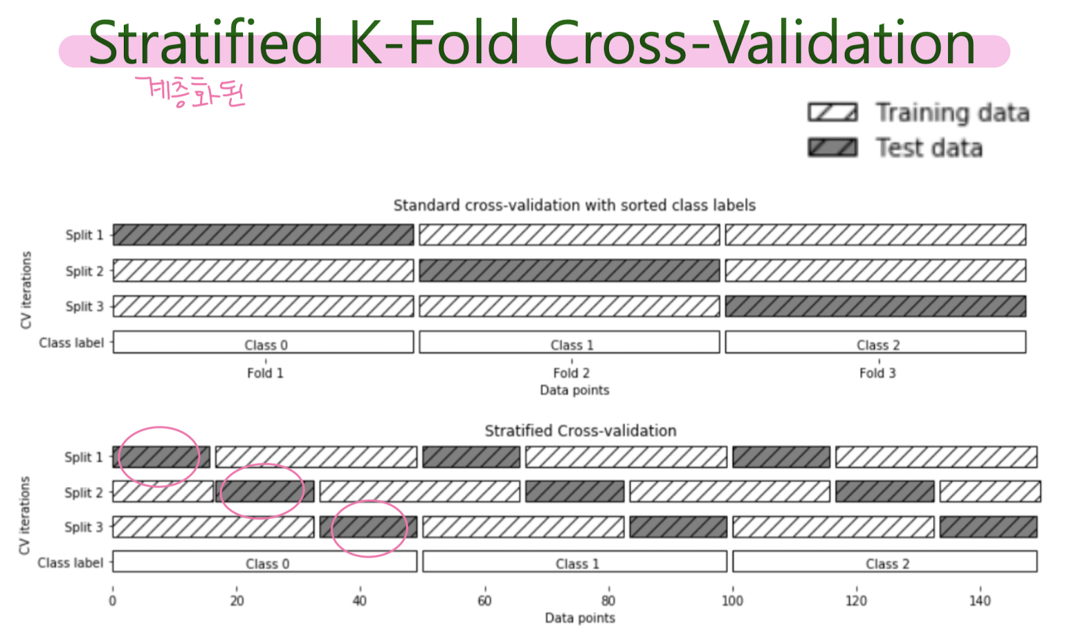
Evaluating Machine Learning Models Using Cross-Validation

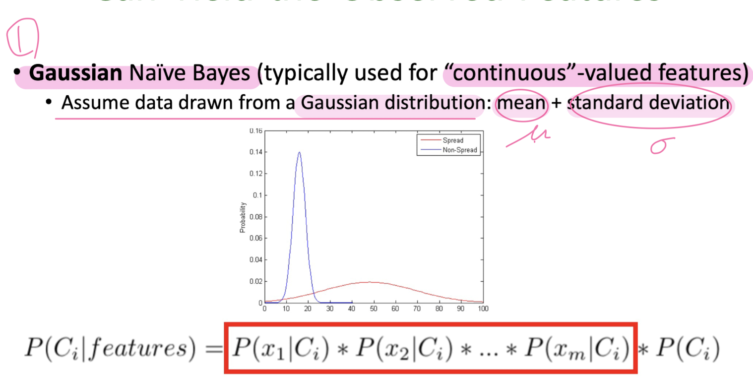
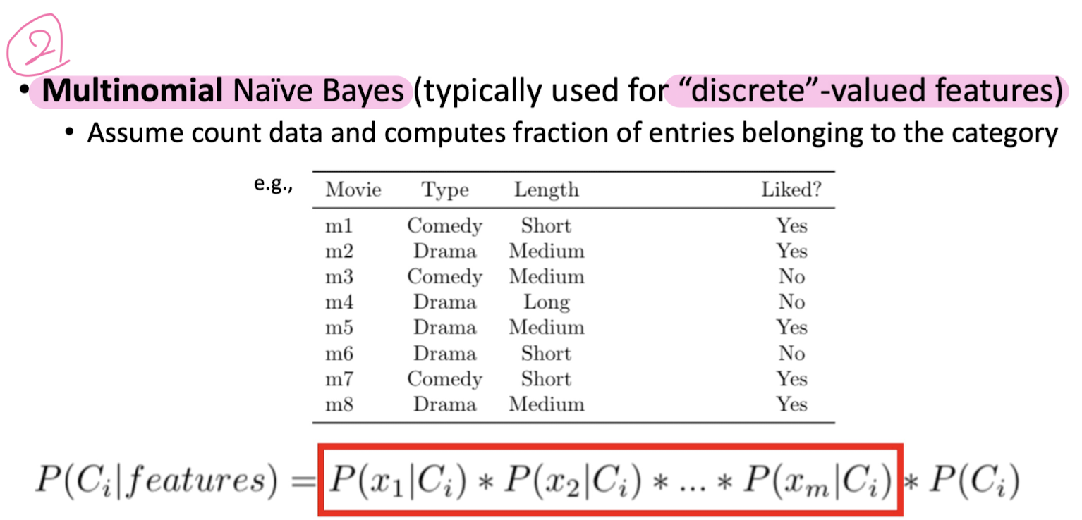
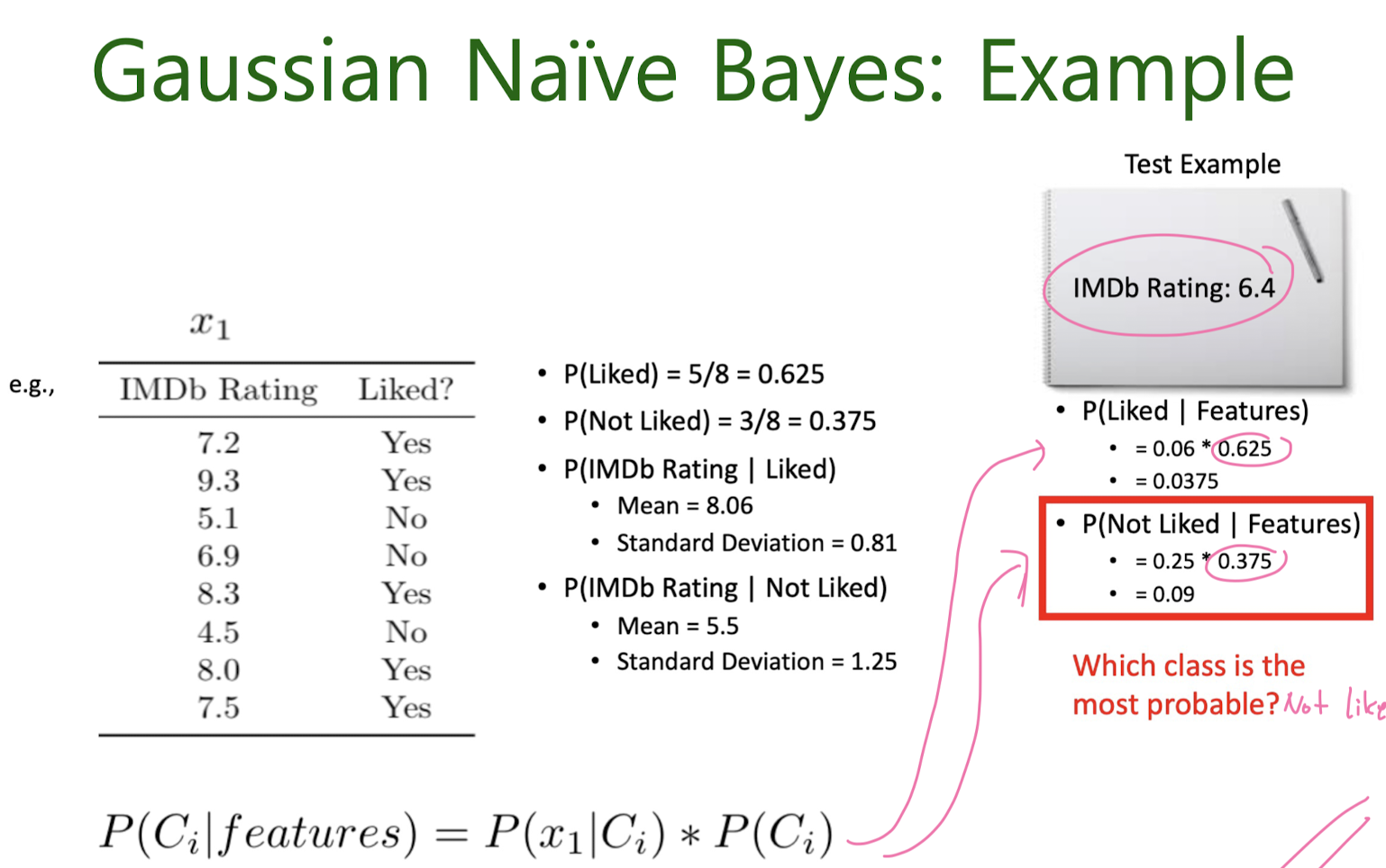
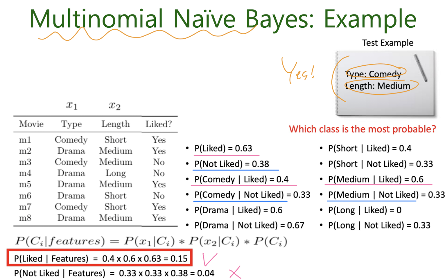
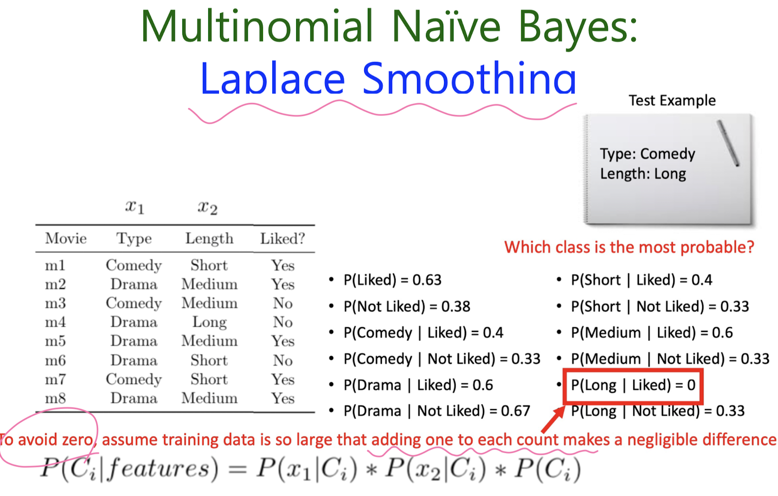
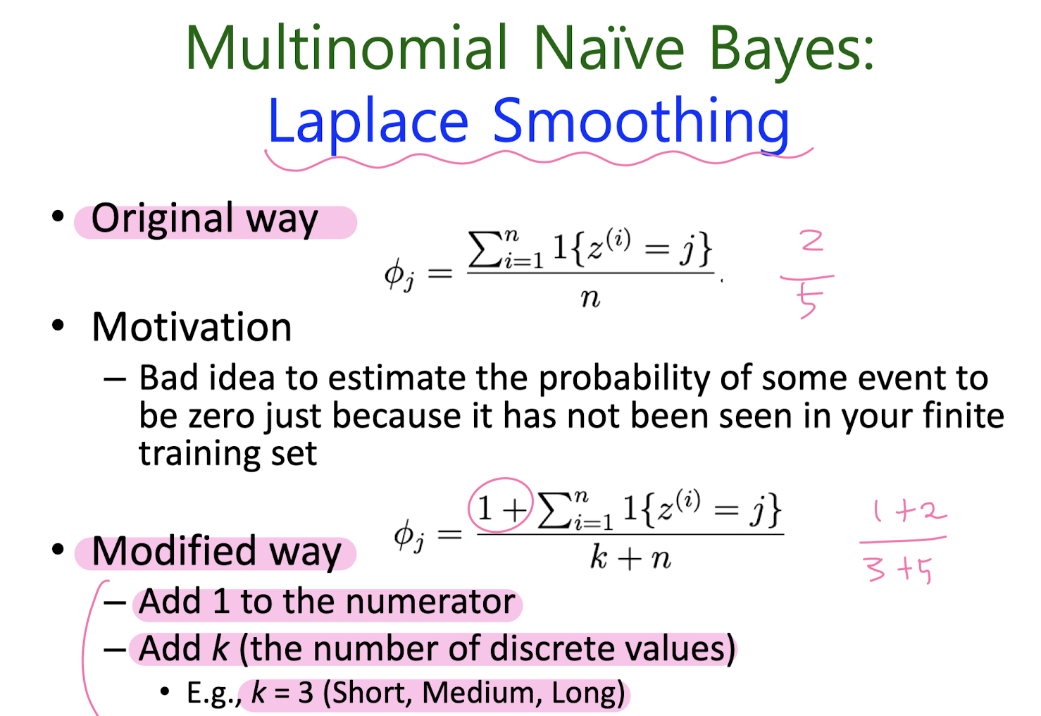
5-1. Naïve Bayes
Background
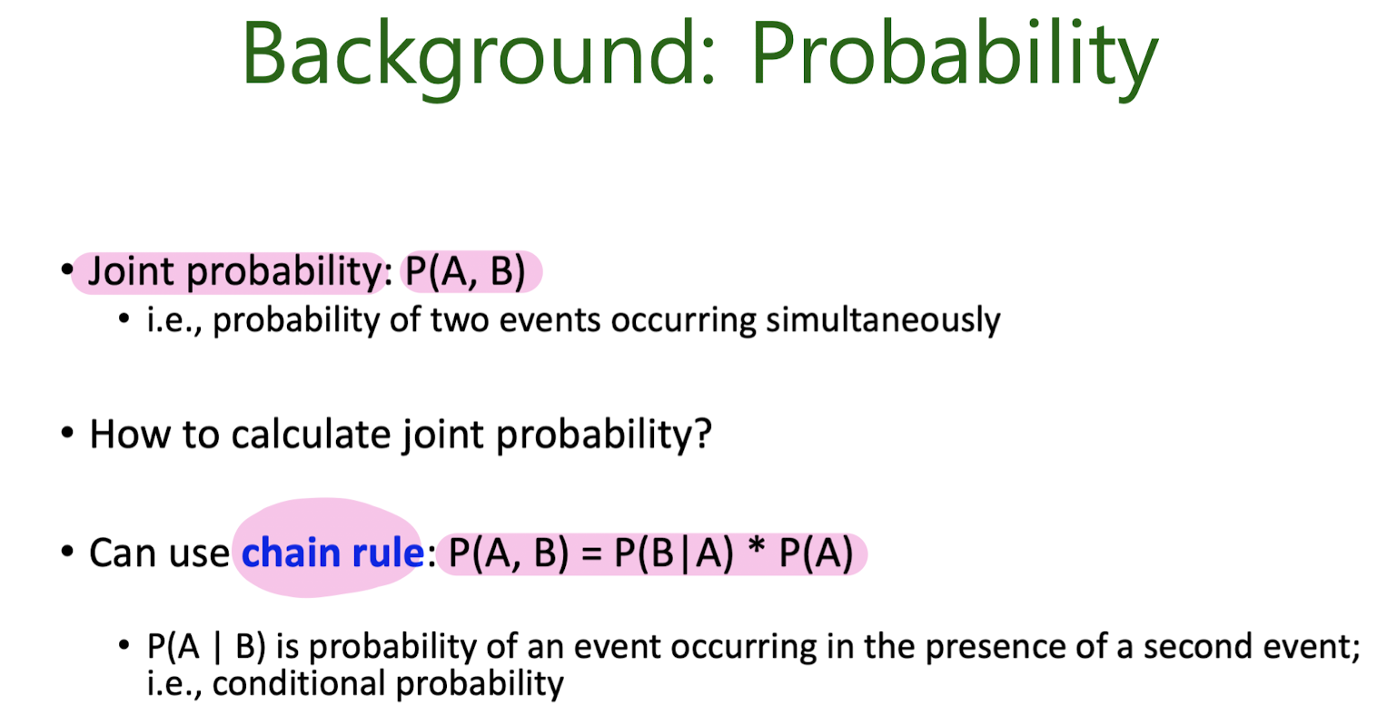
 )
)
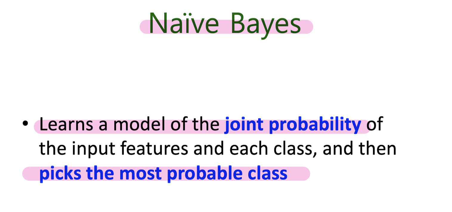
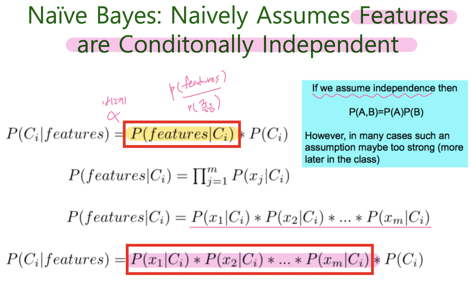
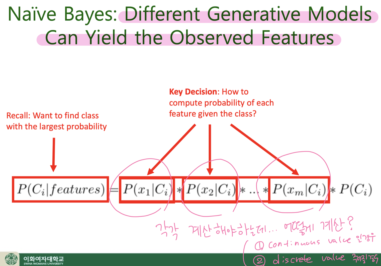
Naïve Bayes
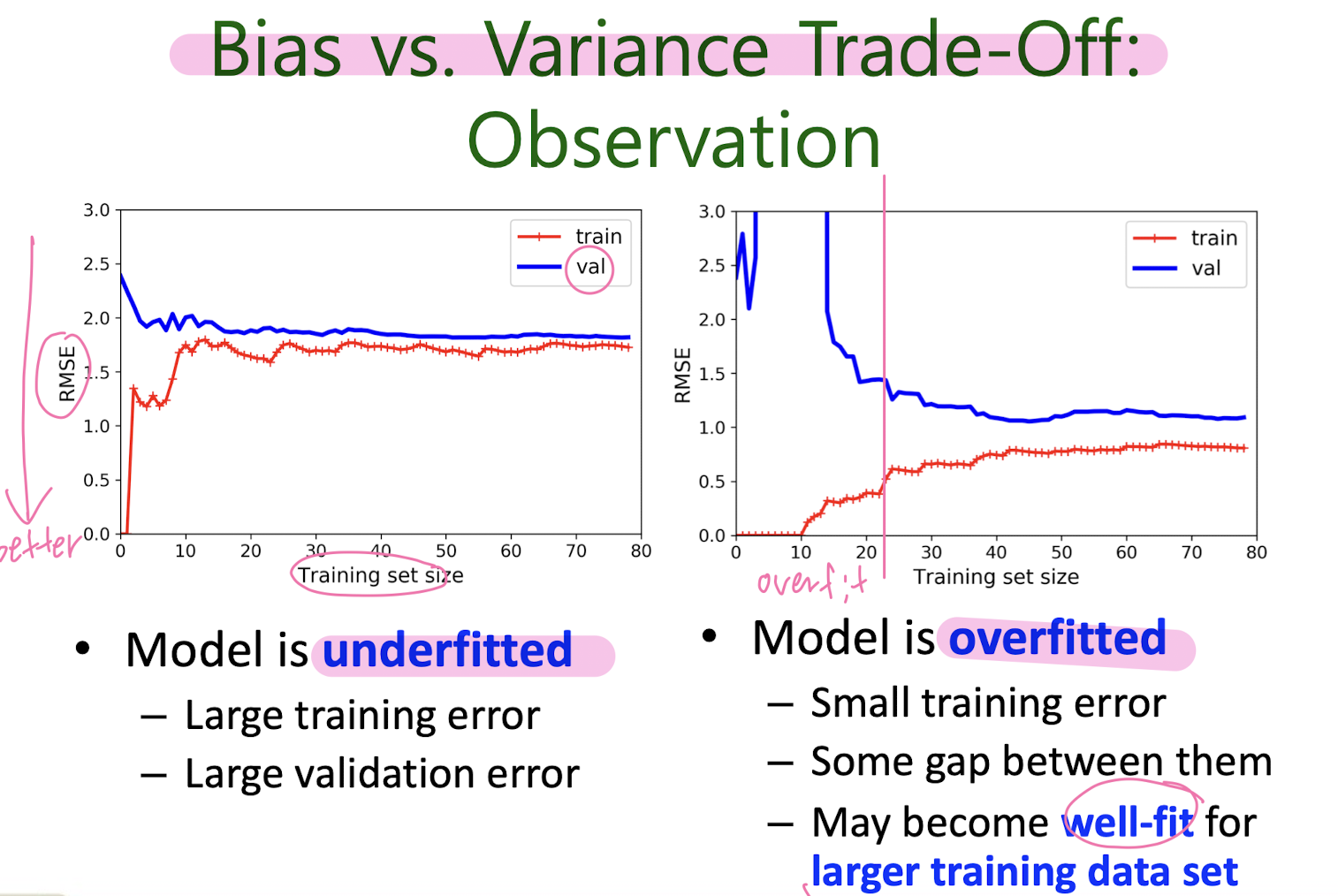
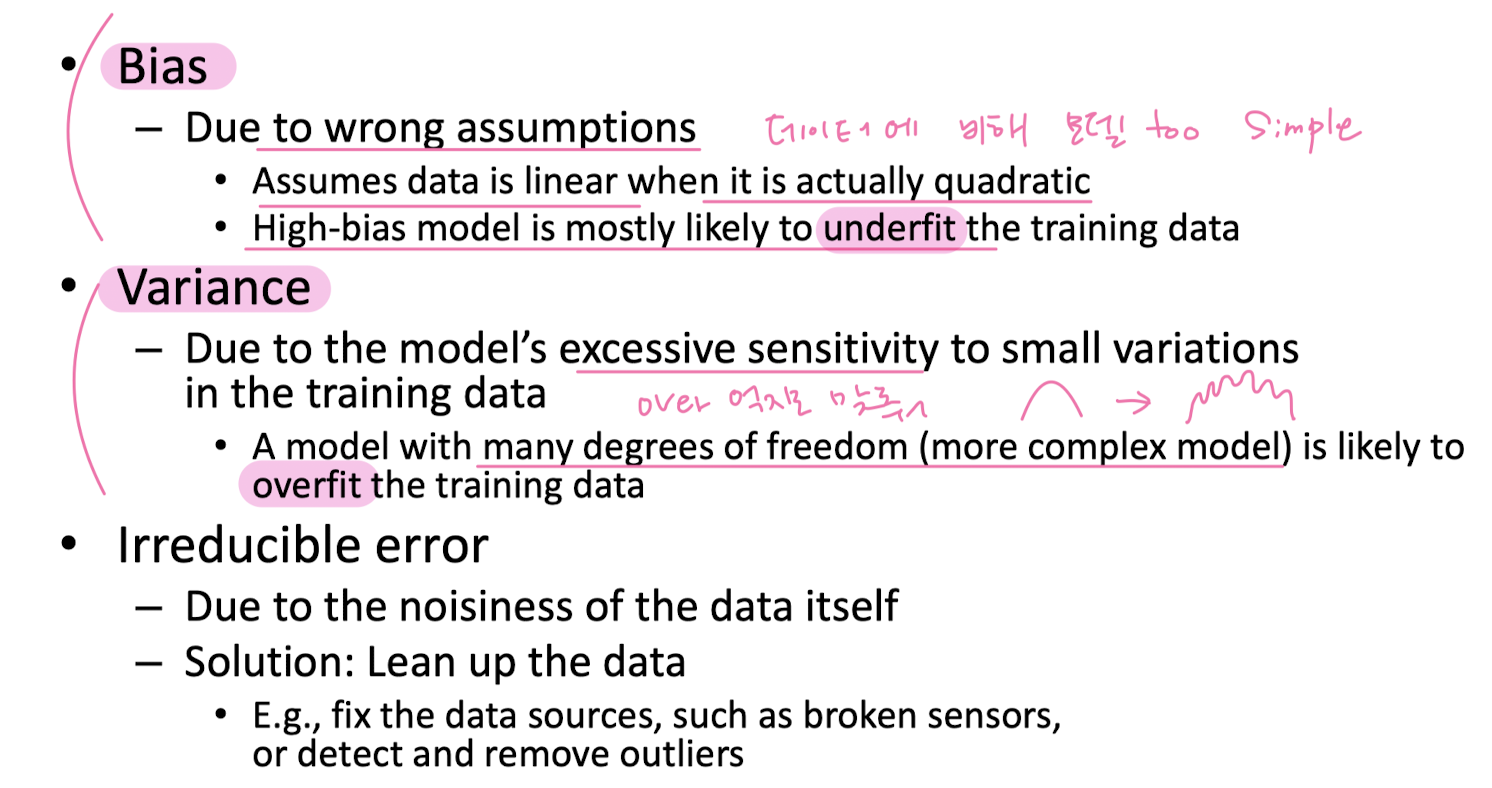
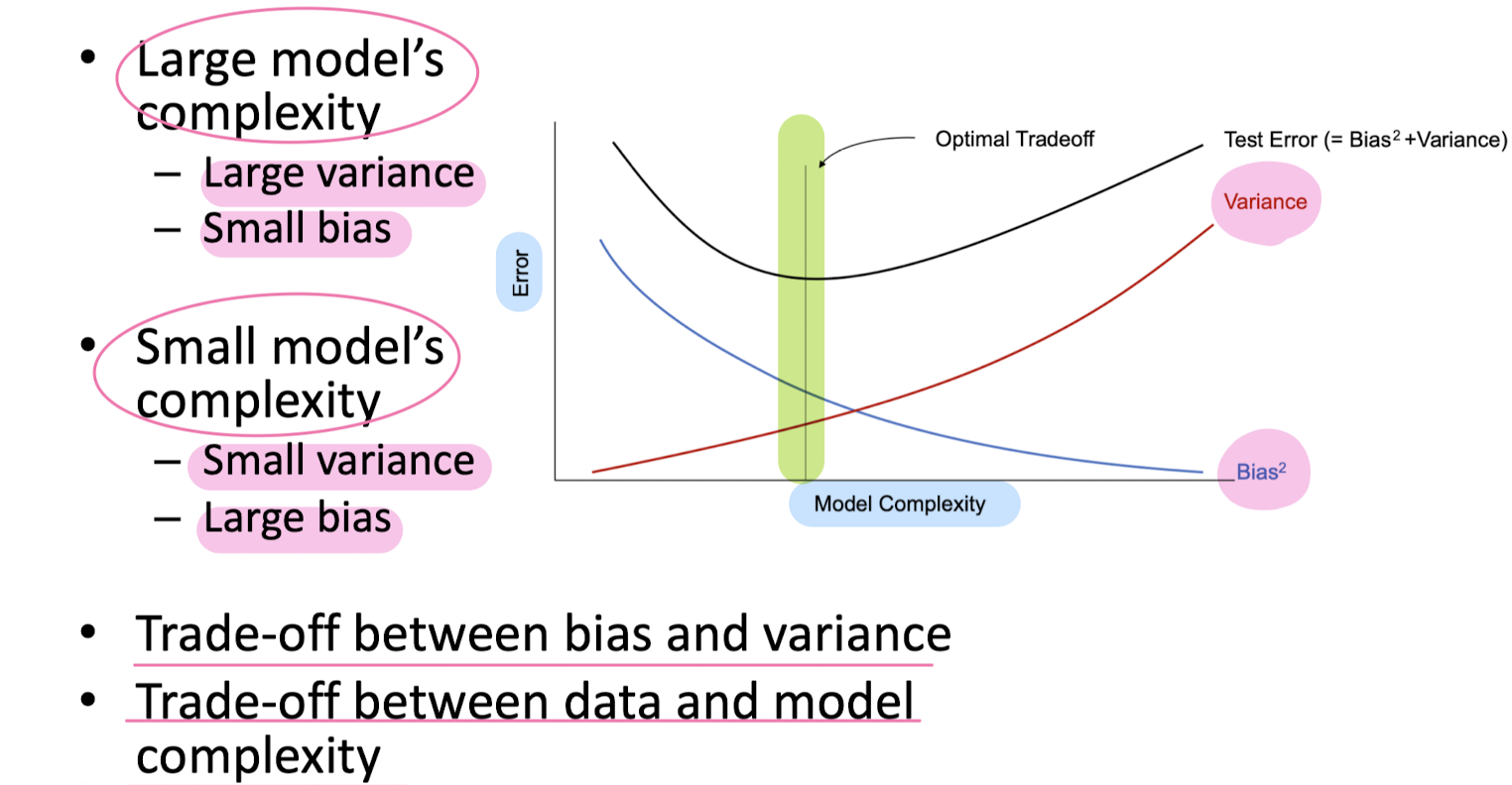
Bias vs. Variance
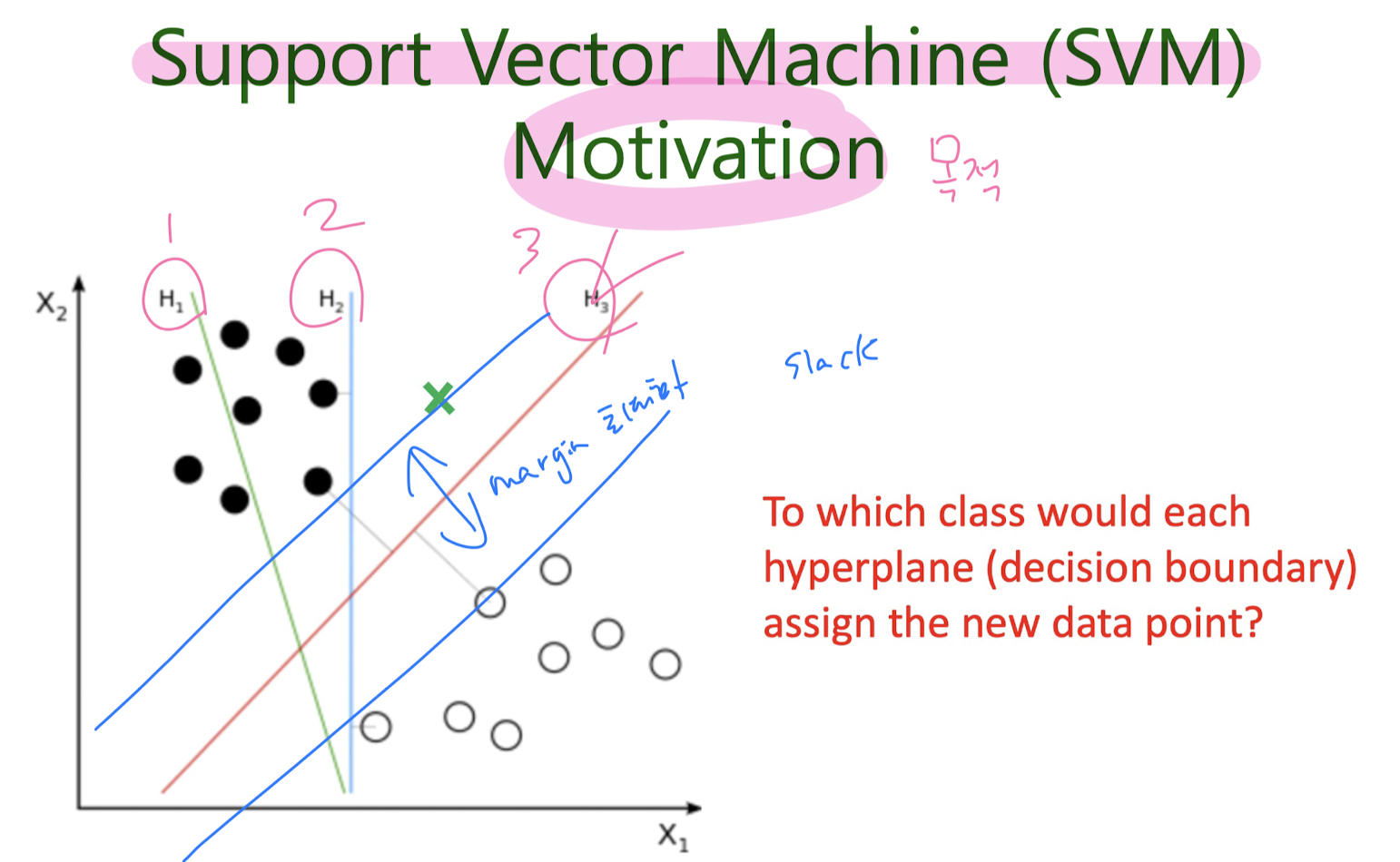
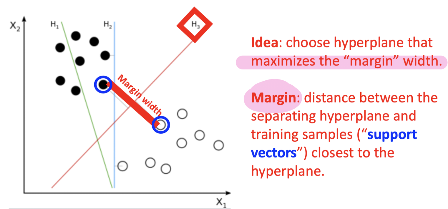
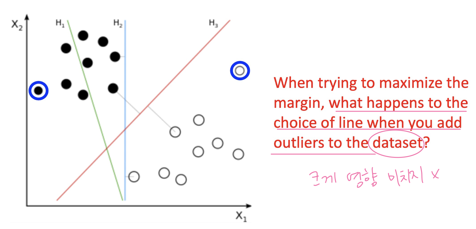
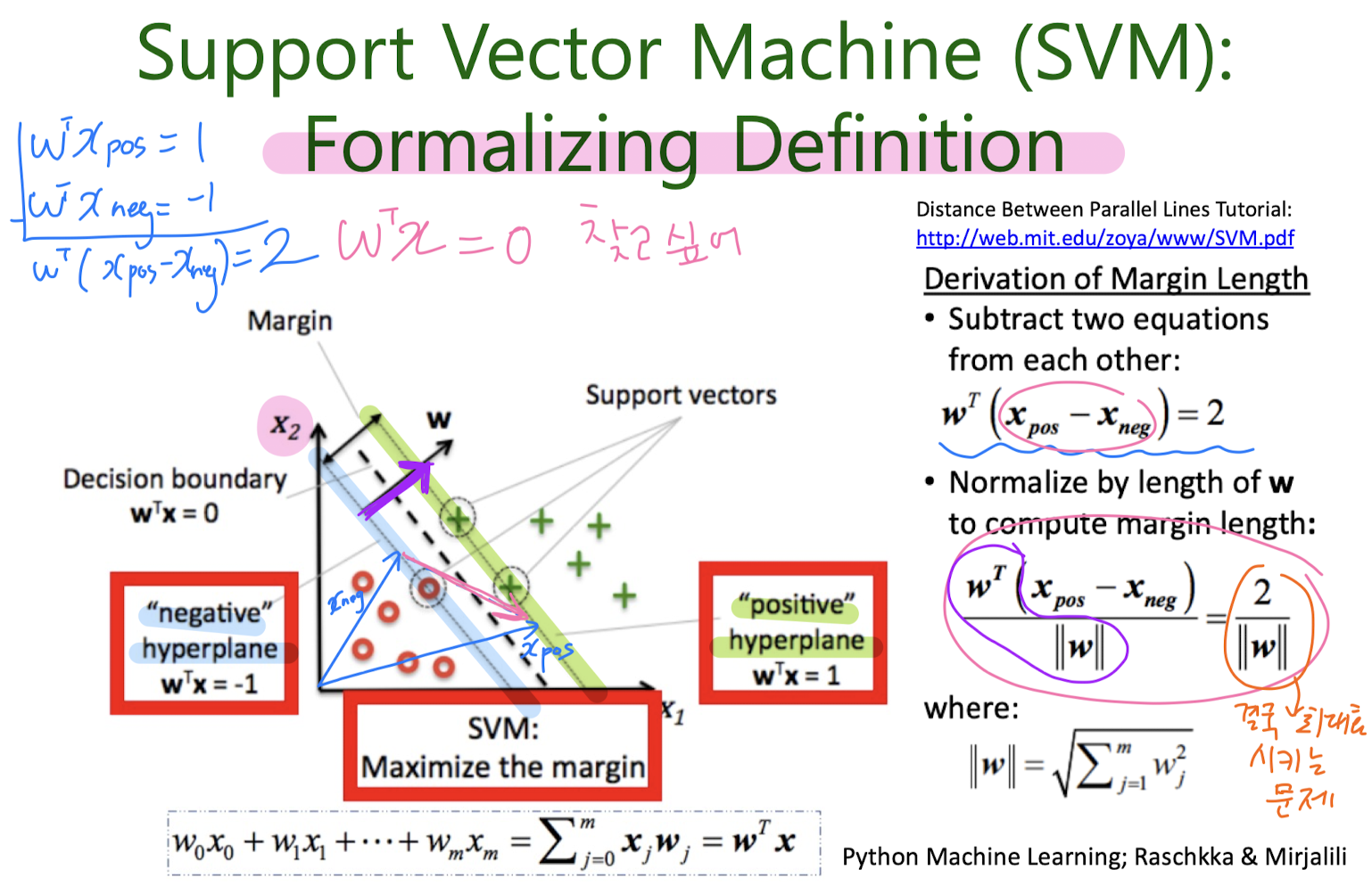
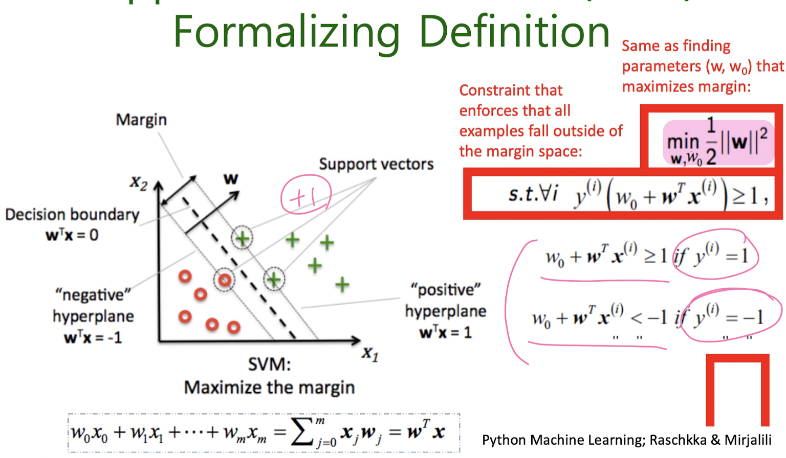
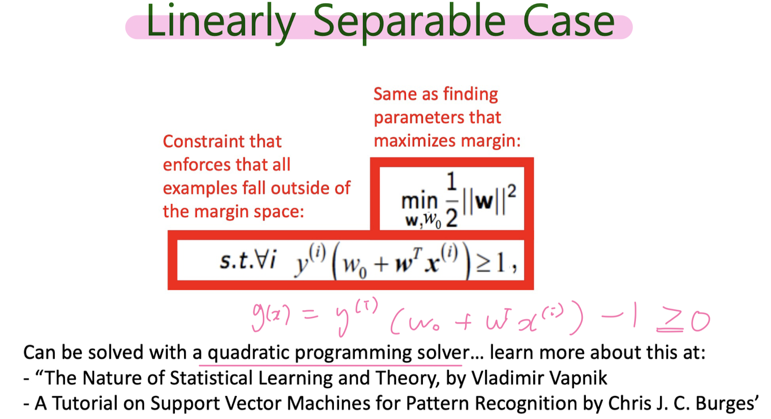
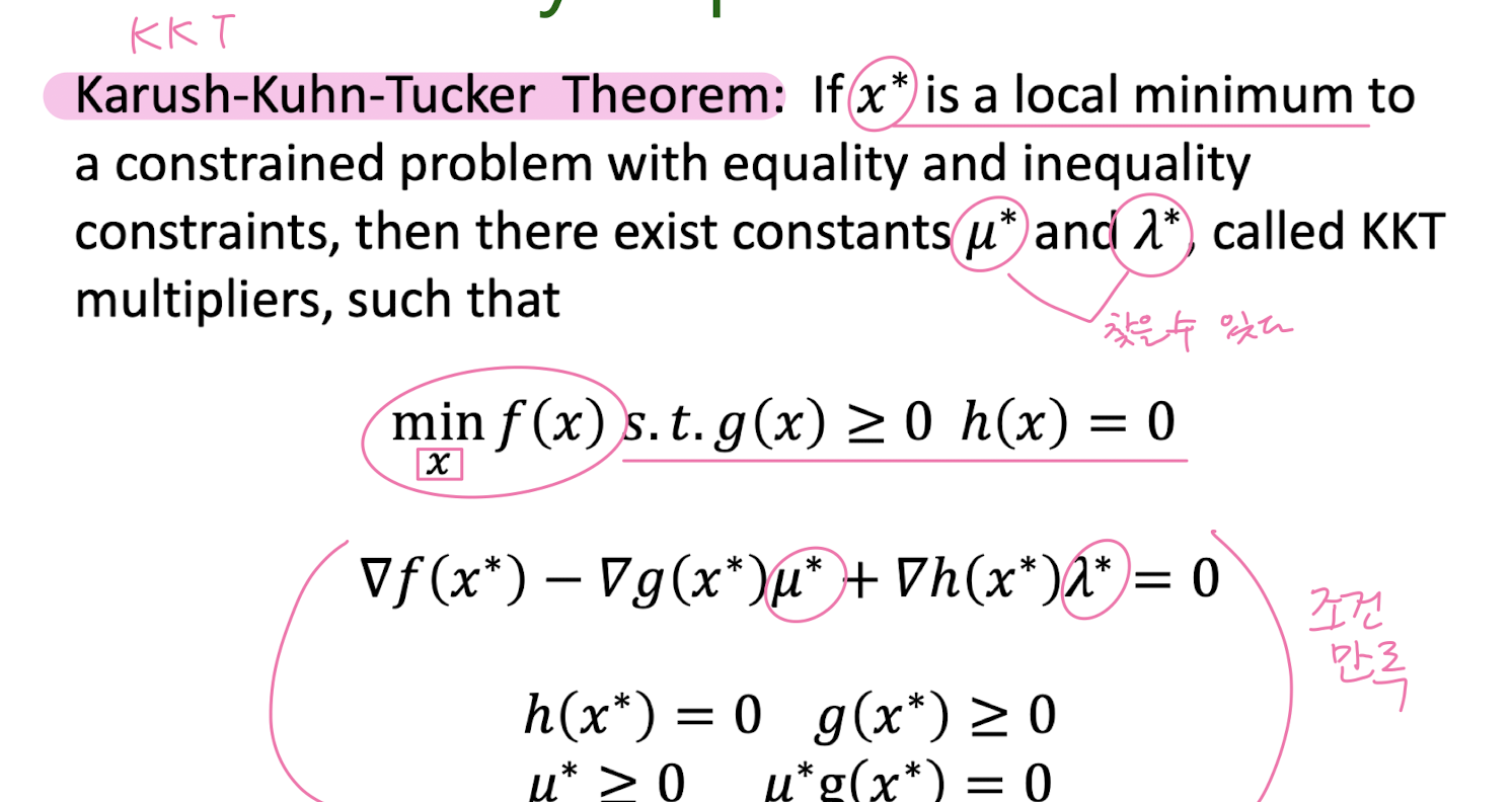
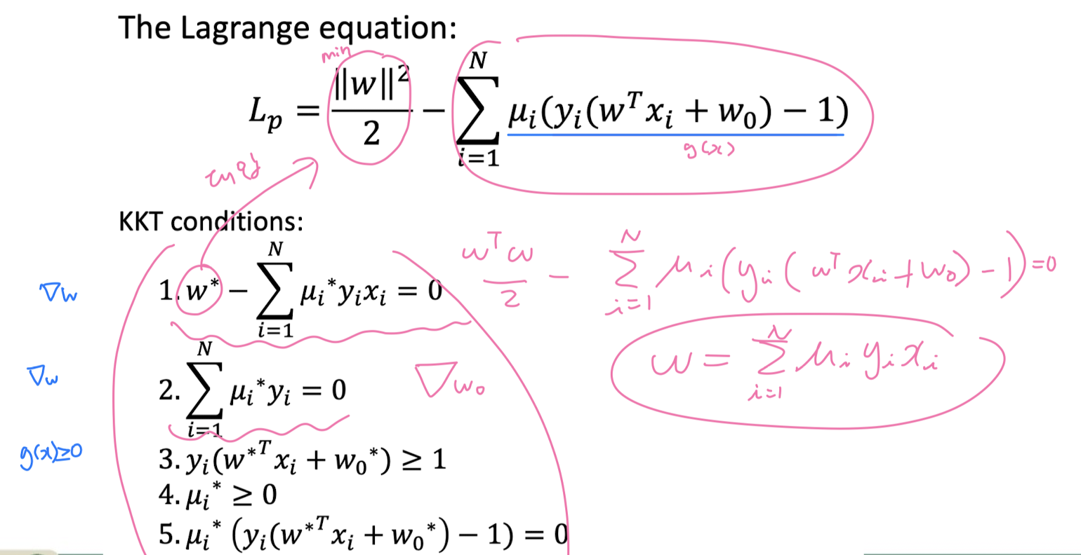
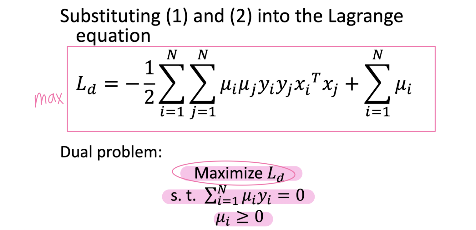
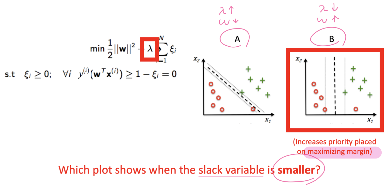
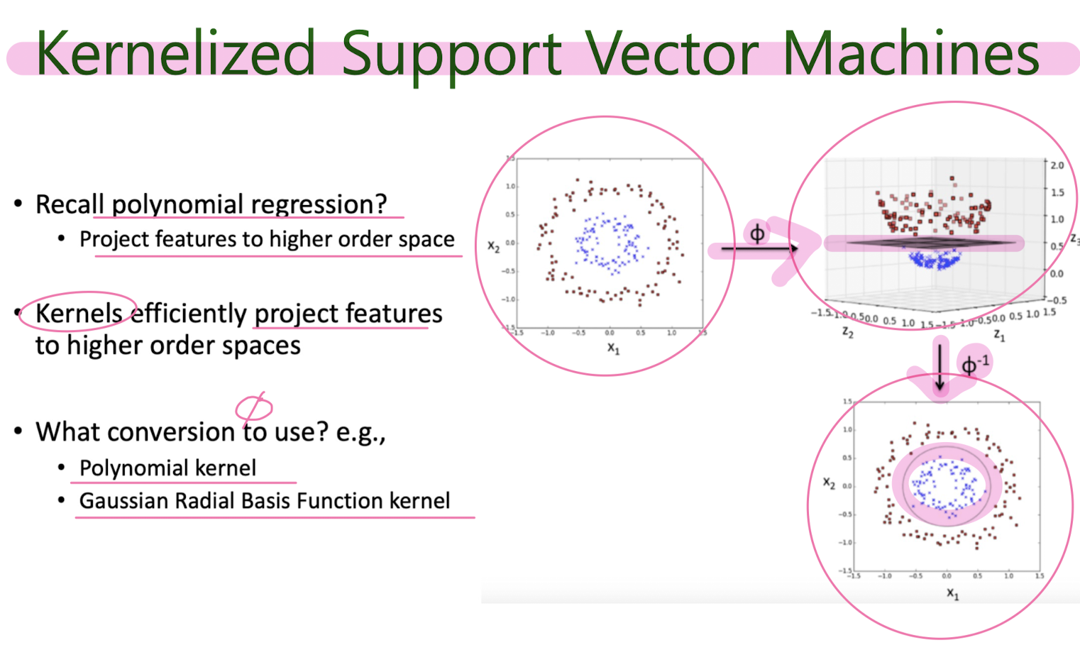
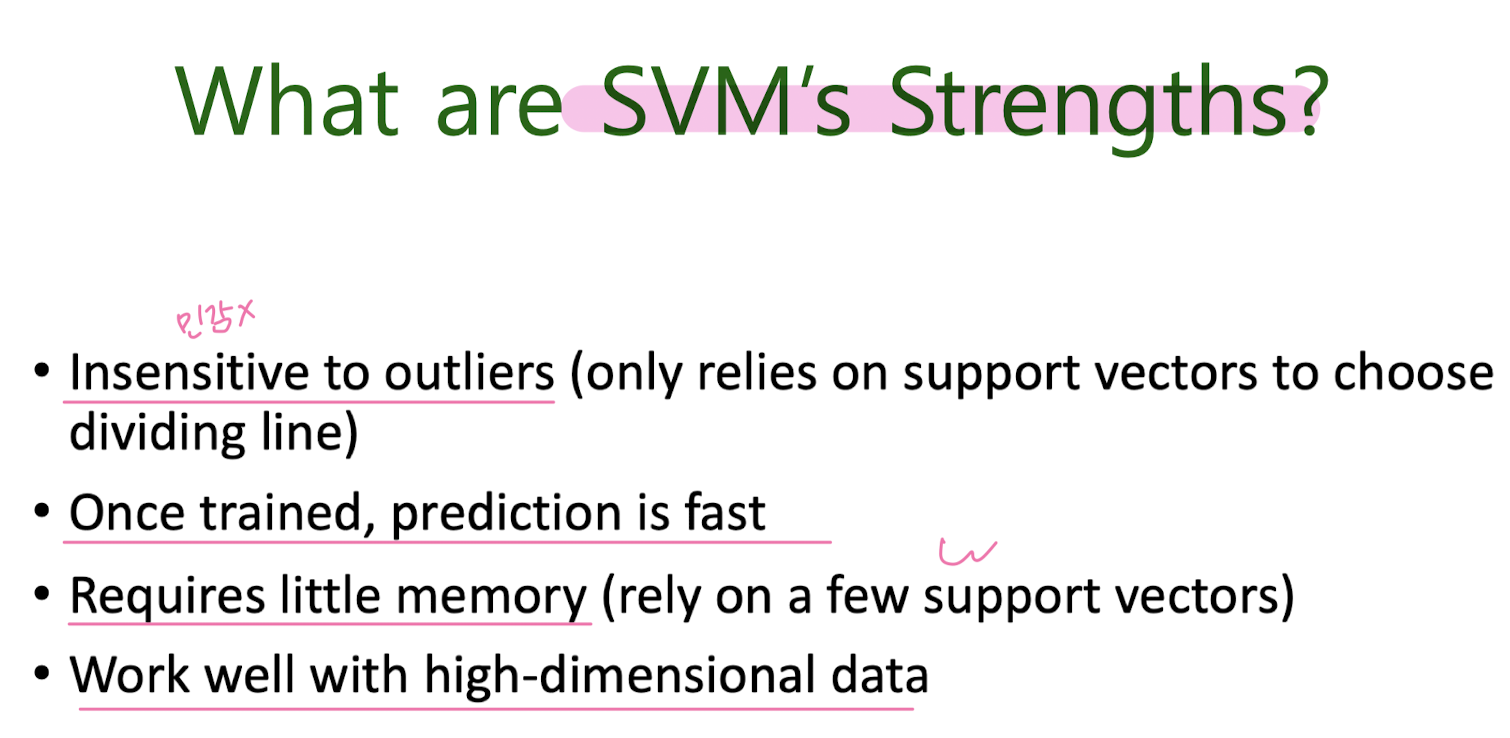
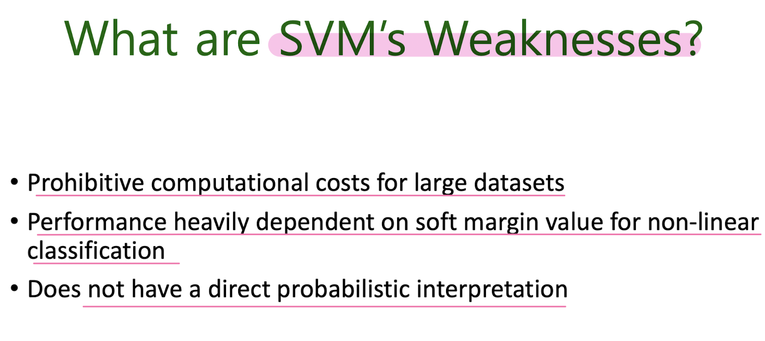
5-2. Support Vector Machine (SVM)
만들어진 분류 모델은 데이터가 사상된 공간에서 경계로 표현되는데 SVM 알고리즘은 그 중 가장 큰 폭을 가진 경계를 찾는 알고리즘이다. SVM은 선형 분류와 더불어 비선형 분류에서도 사용될 수 있다. 비선형 분류를 하기 위해서 주어진 데이터를 고차원 특징 공간으로 사상하는 작업이 필요한데, 이를 효율적으로 하기 위해 커널 트릭을 사용하기도 한다.
Linearly seperable (Hard- Margin Classificattion)
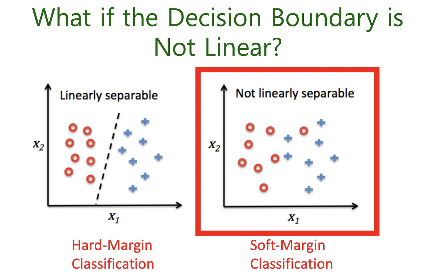
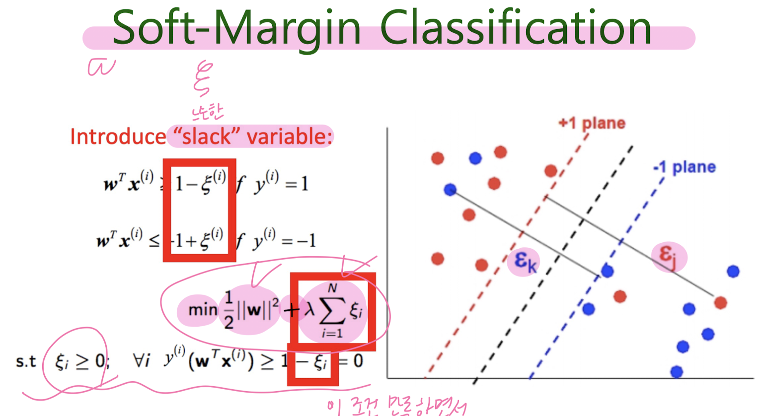
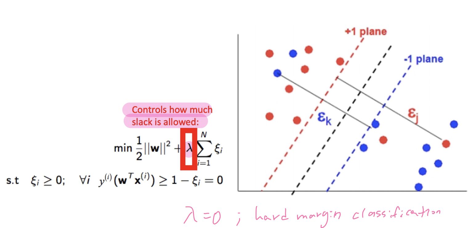
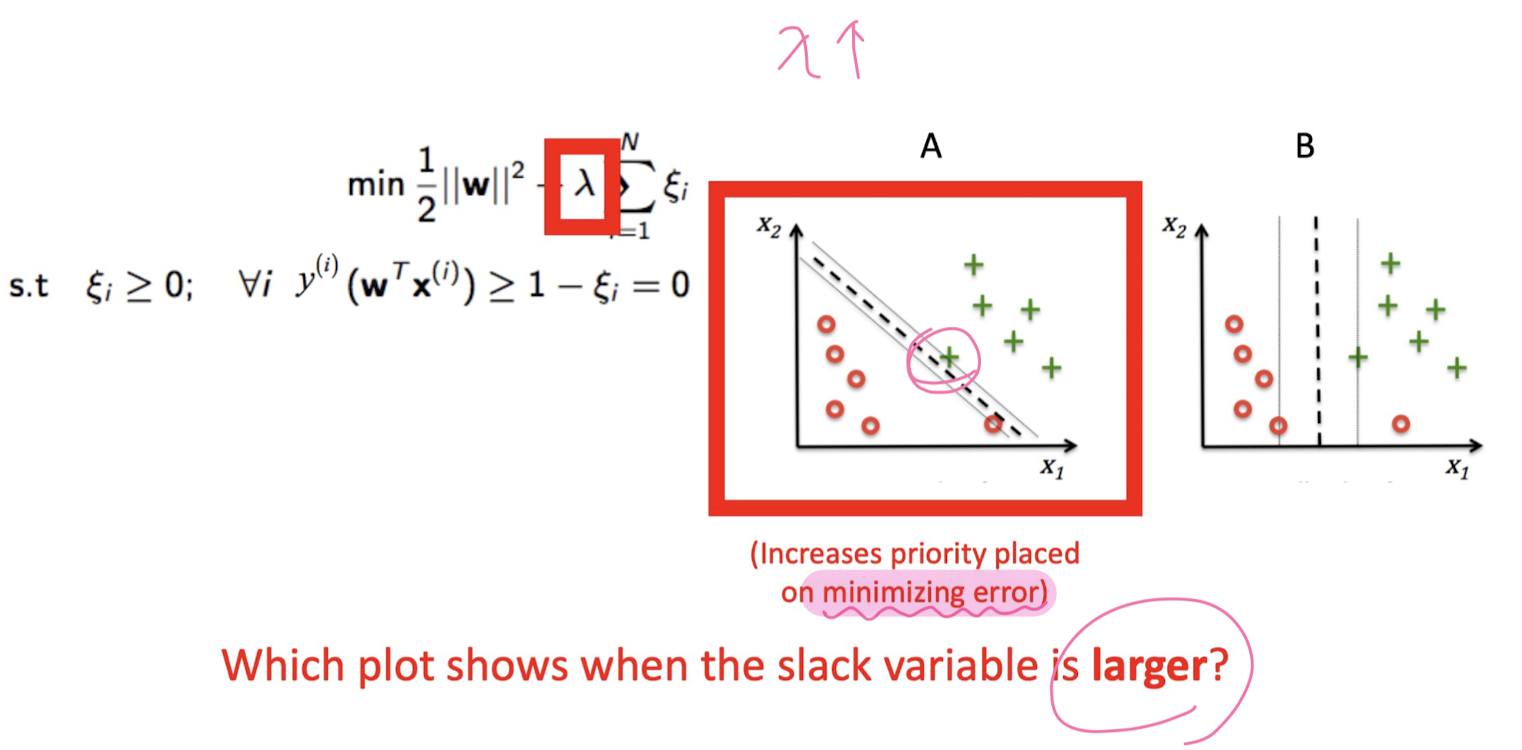
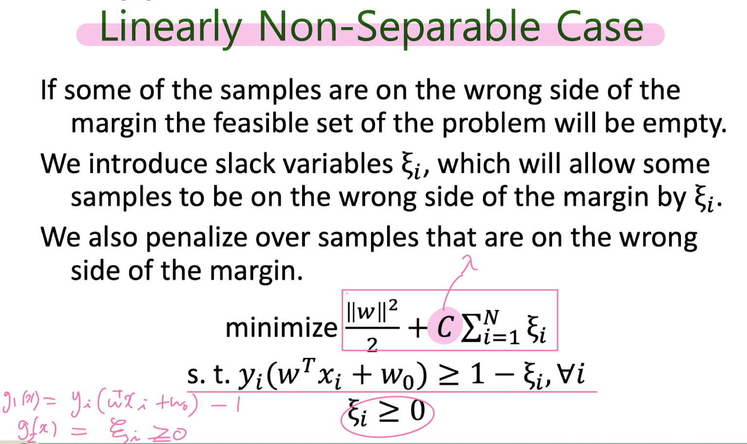
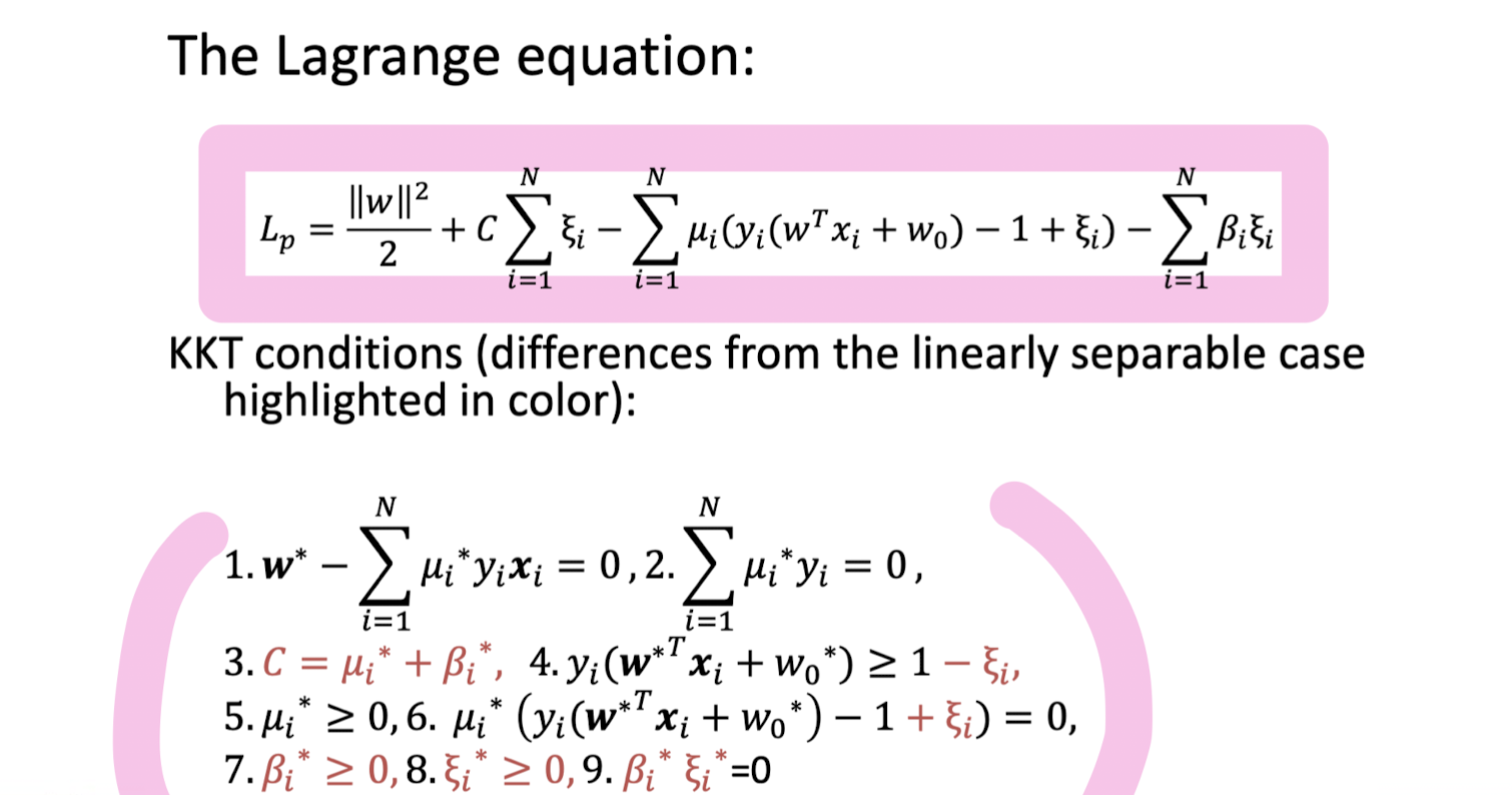
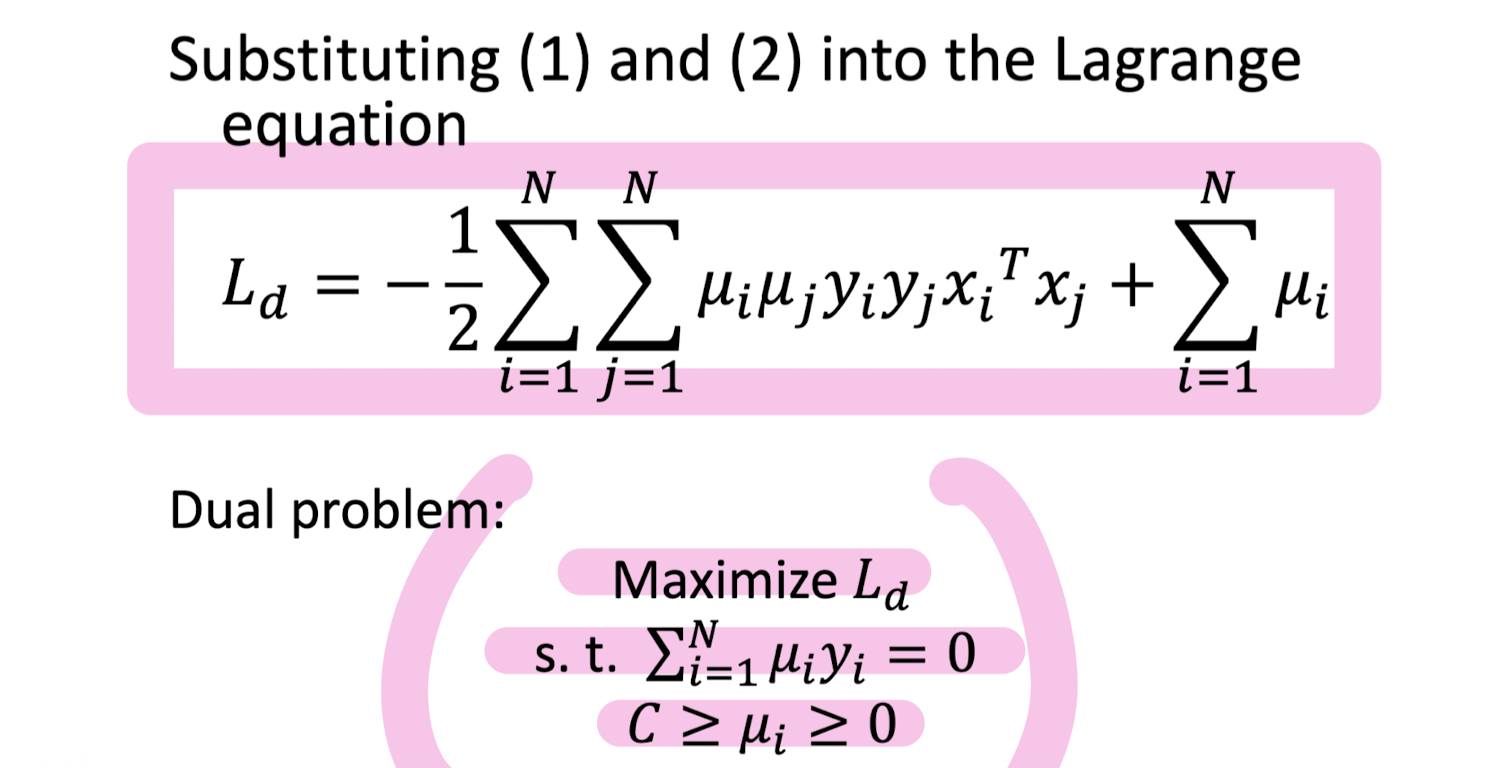
Not Linearly seperable (Soft-Margin Classificattion)
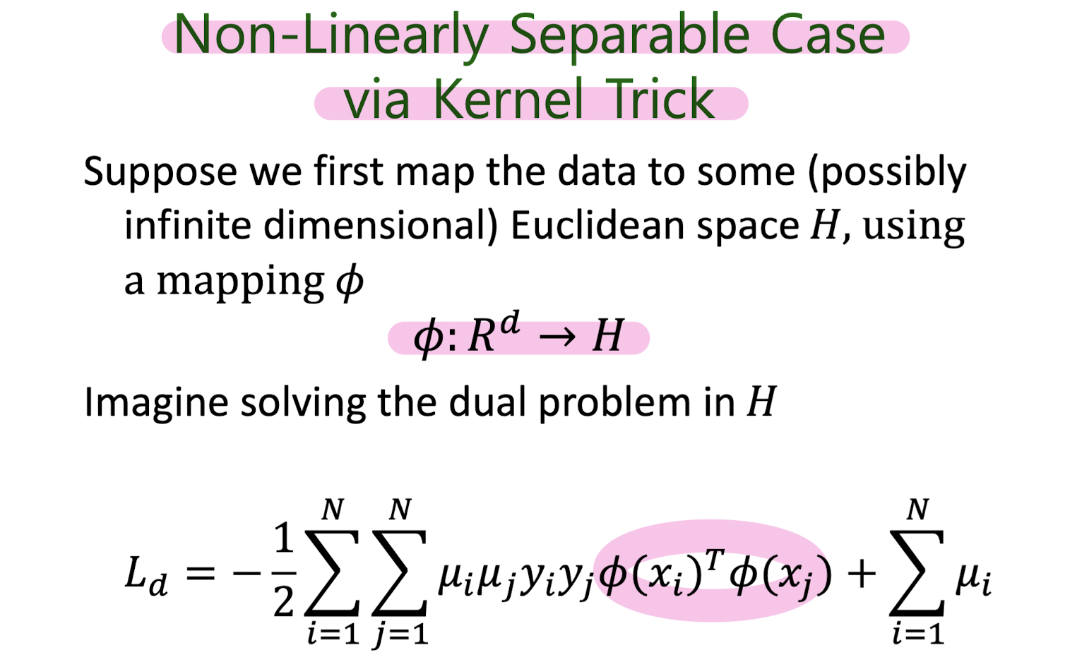
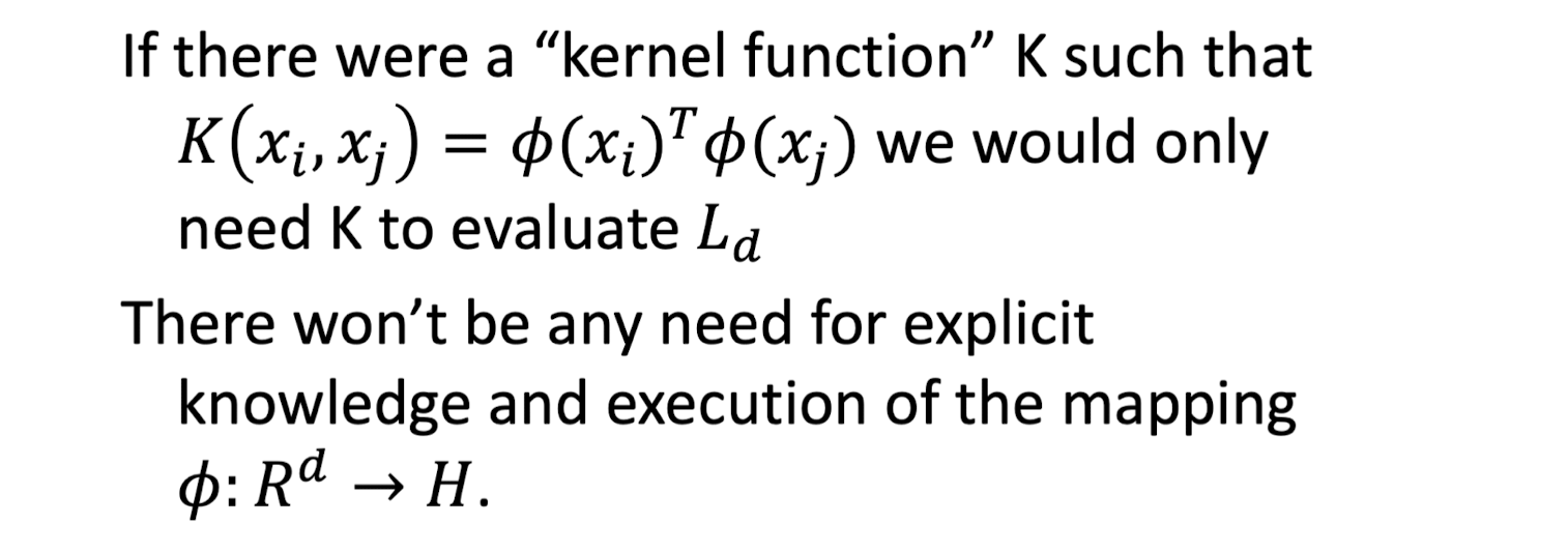
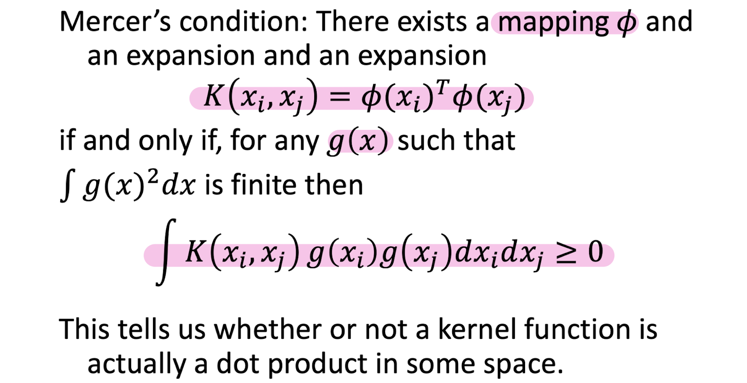
Not Linearly seperable - kernelized SVM
SVM 장단점
6. Unsupervised learning: Clustering
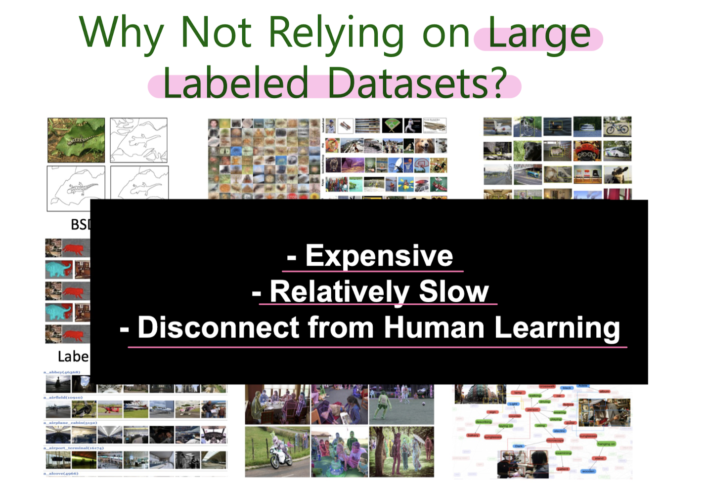
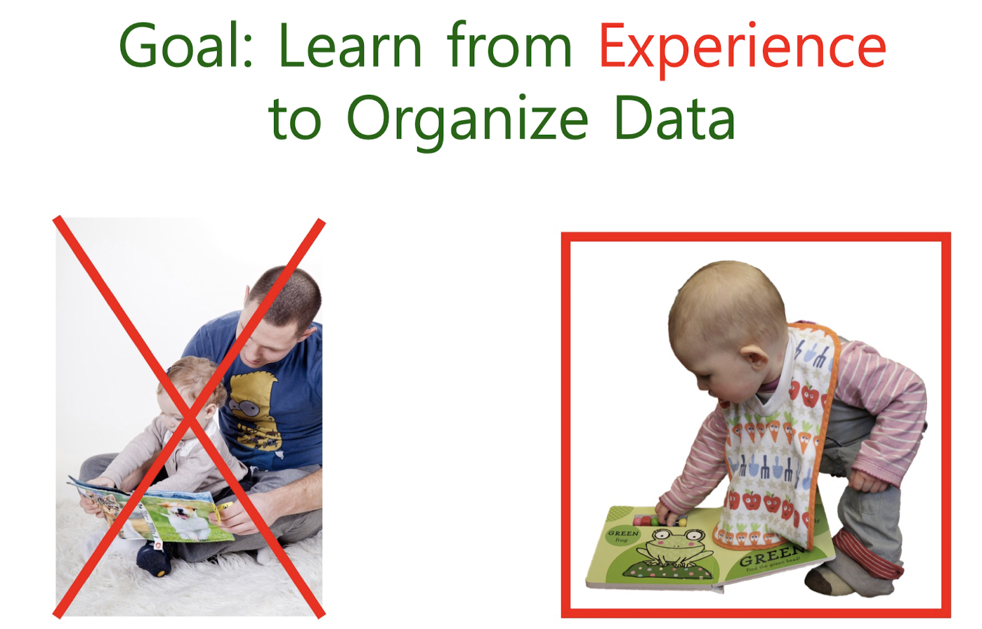
Motivation: Unsupervised learning & Clustering
Real-World Applications:
- Customer Segmentation
- Recommendations
- Socila Network Analysis
- Fraud Detection
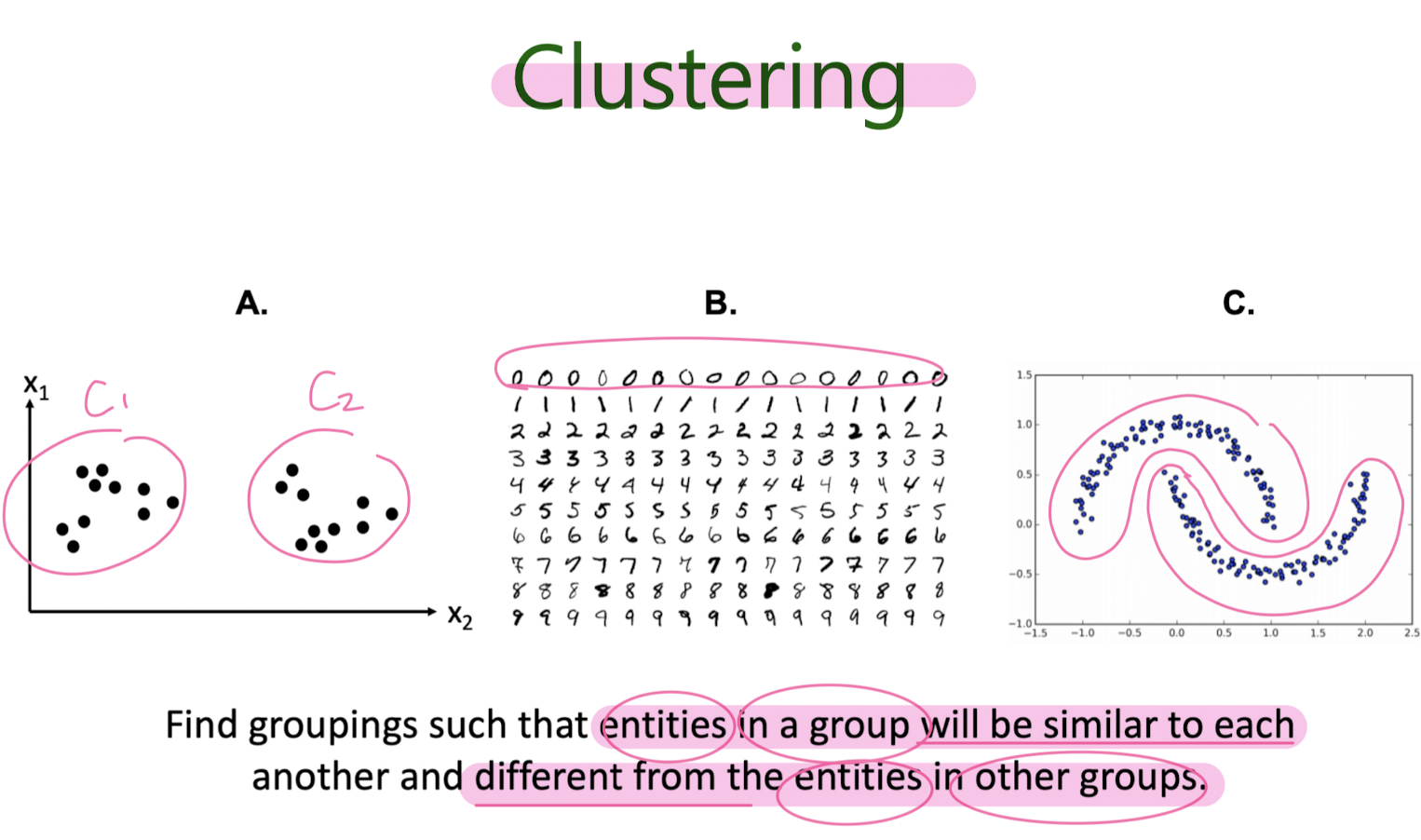
Clustering
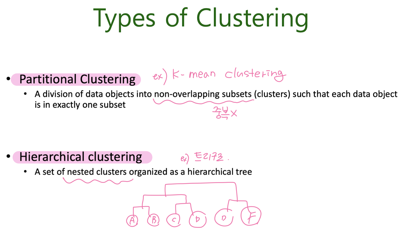
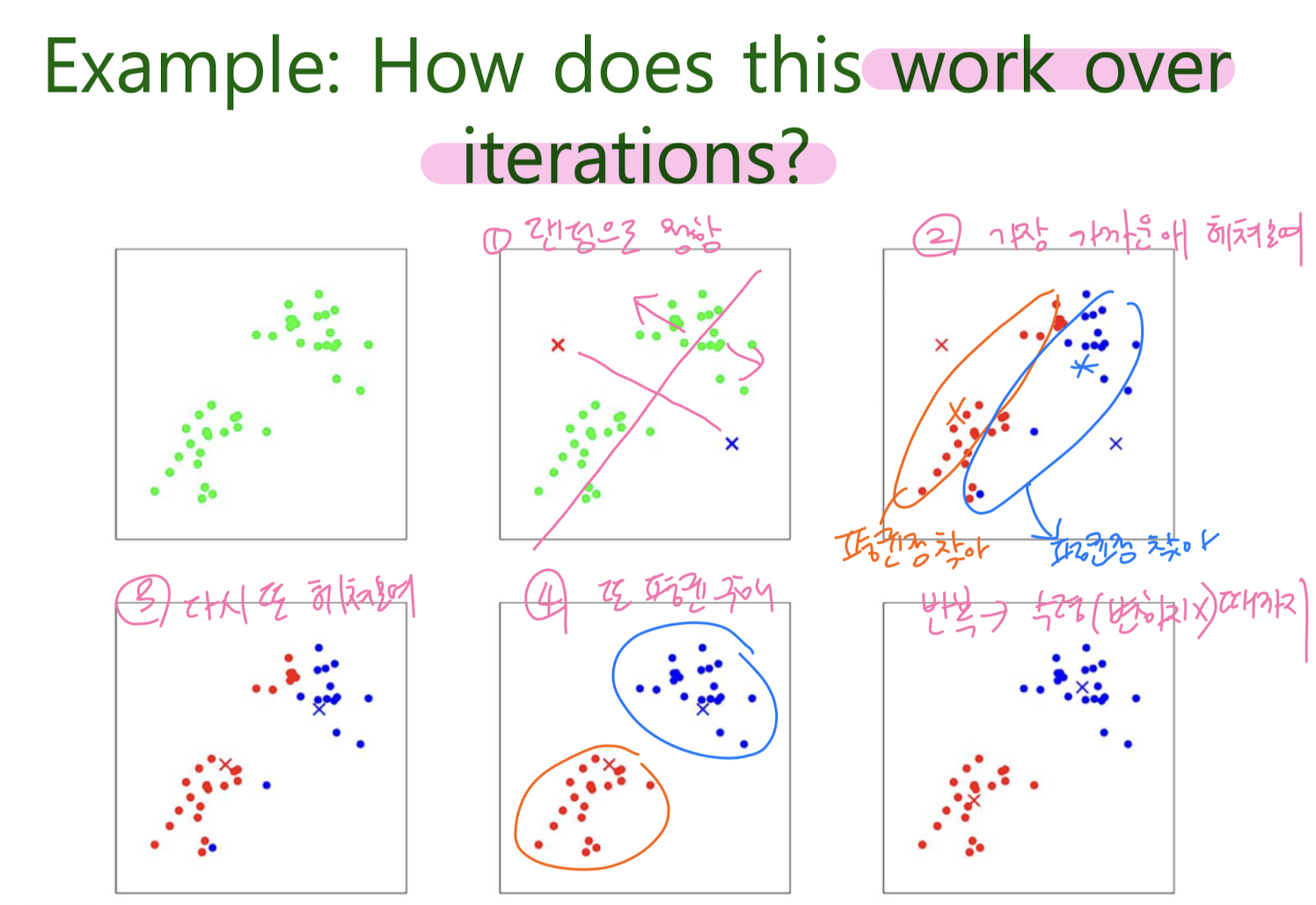
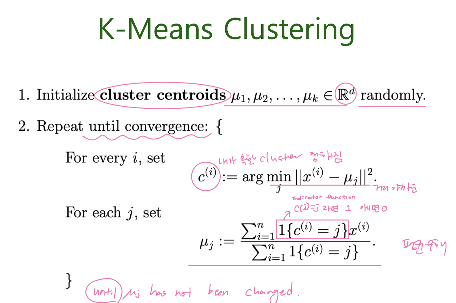
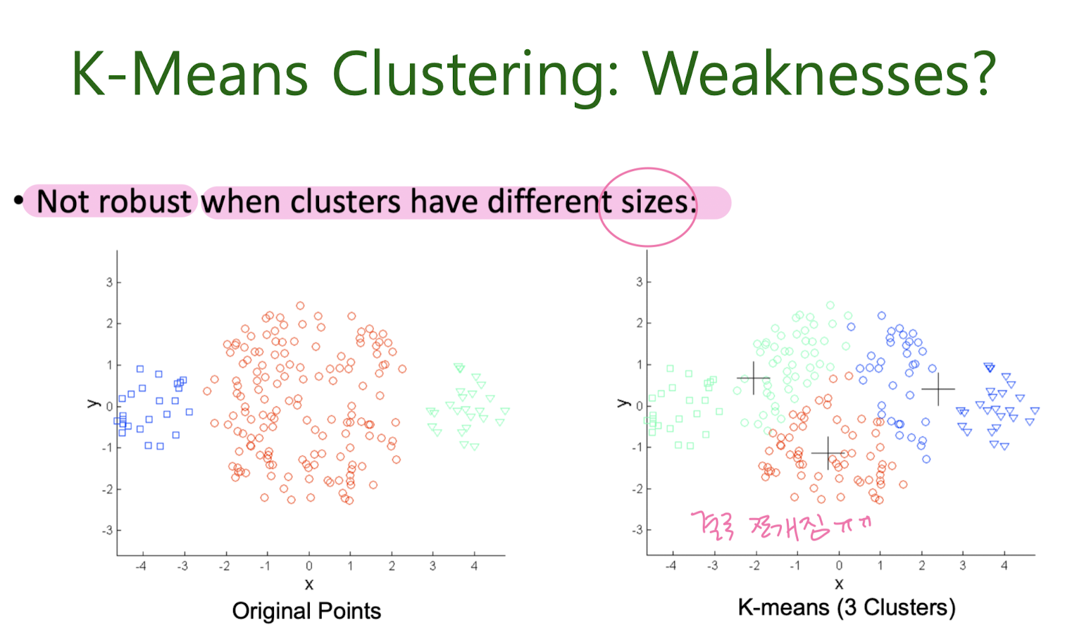
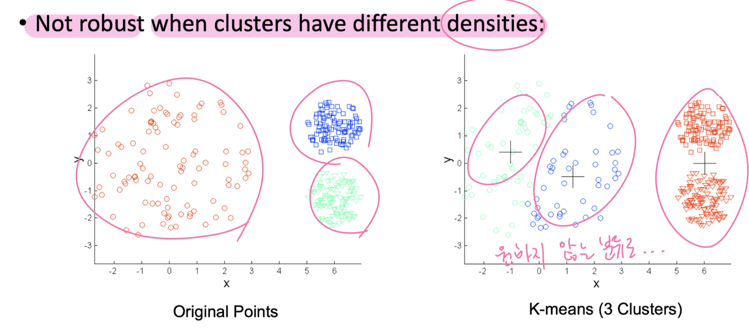
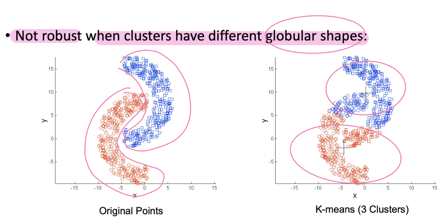
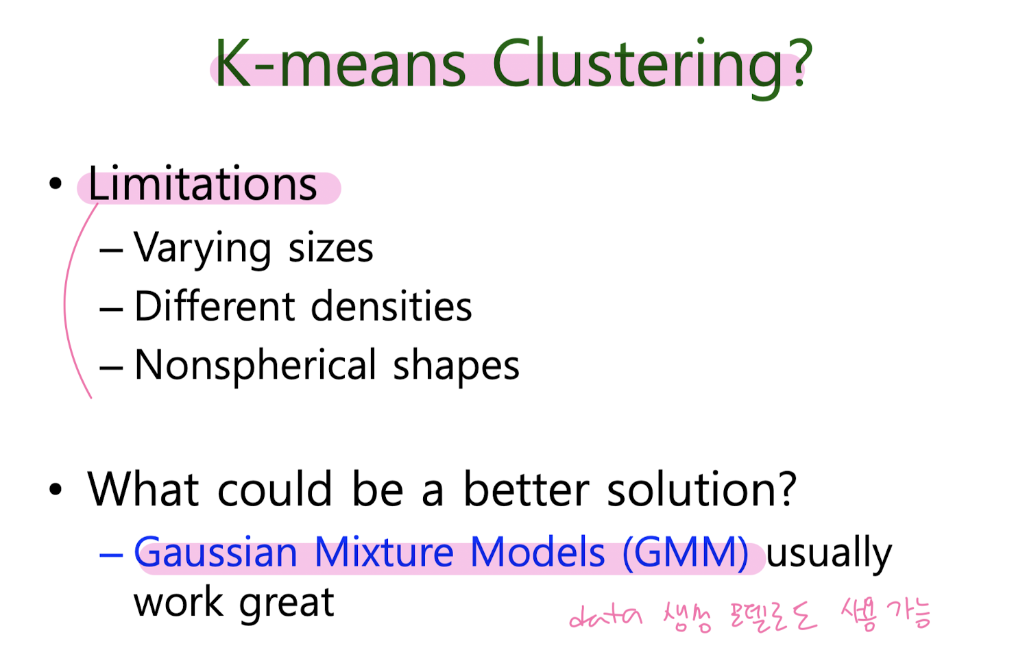
K-Means Clustering
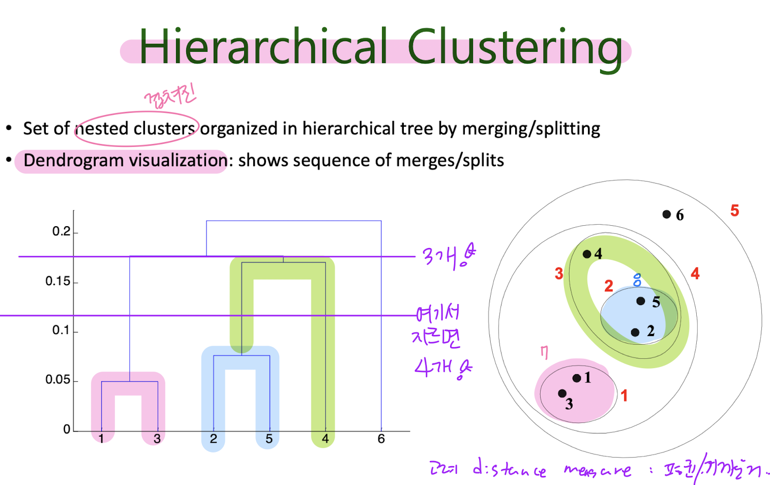
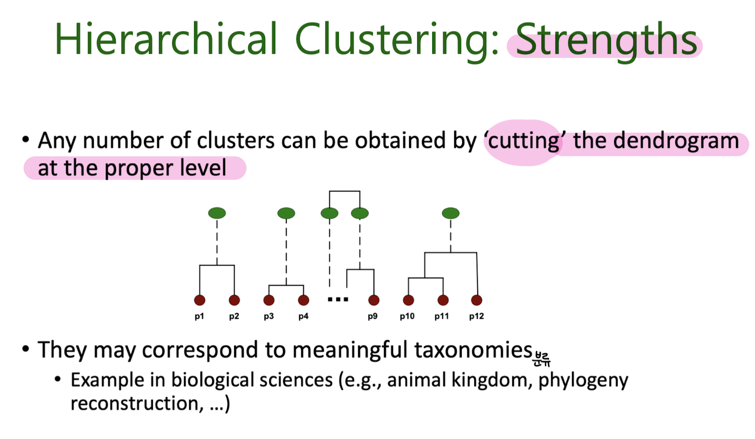
Hierarchical Clustering
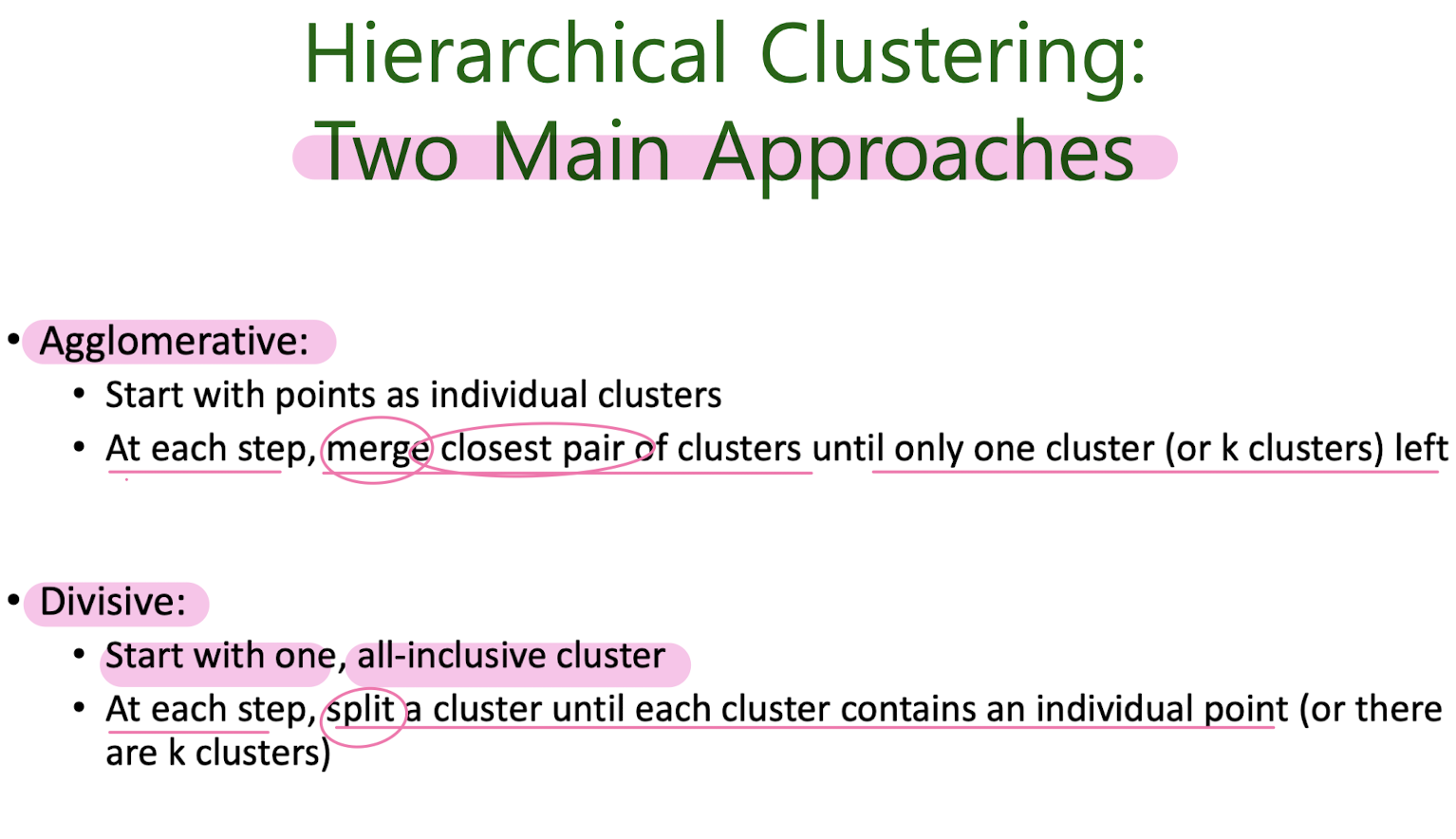
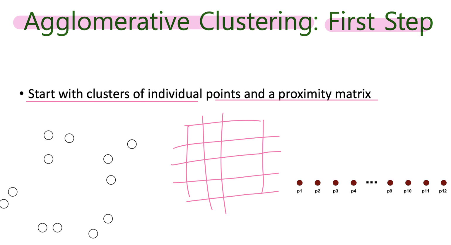
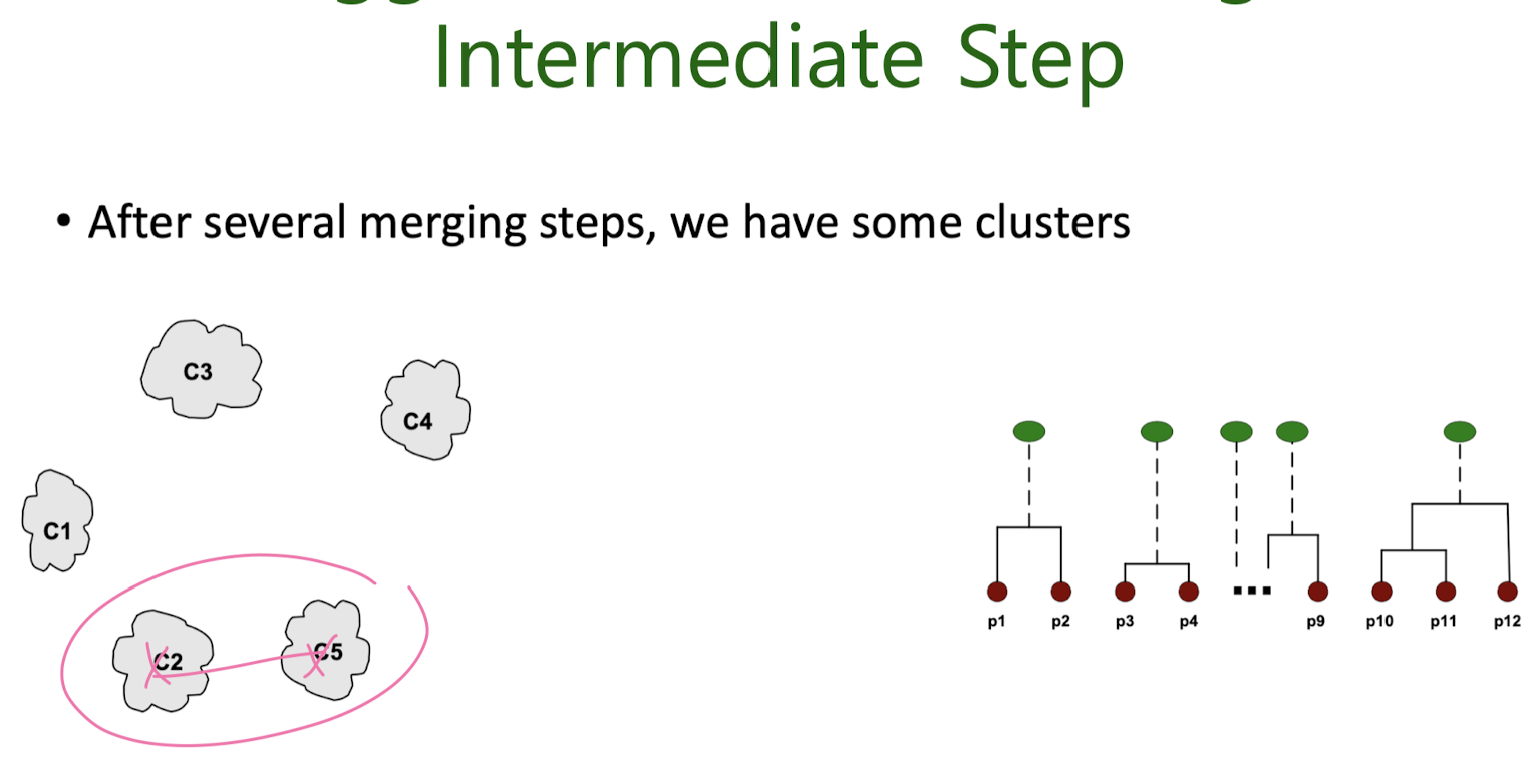
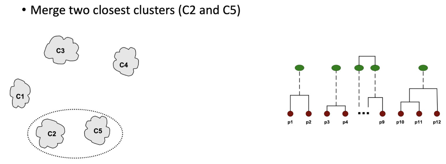
Agglomerative
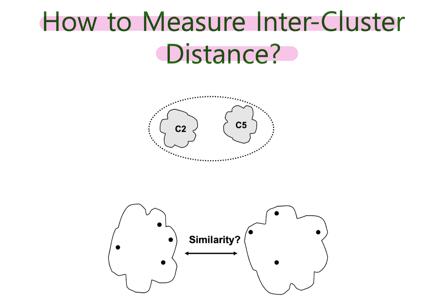
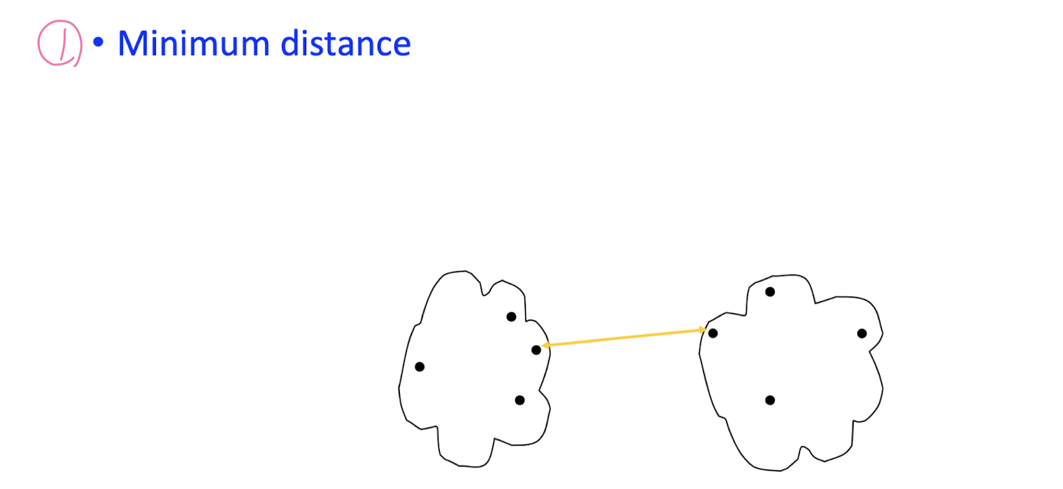
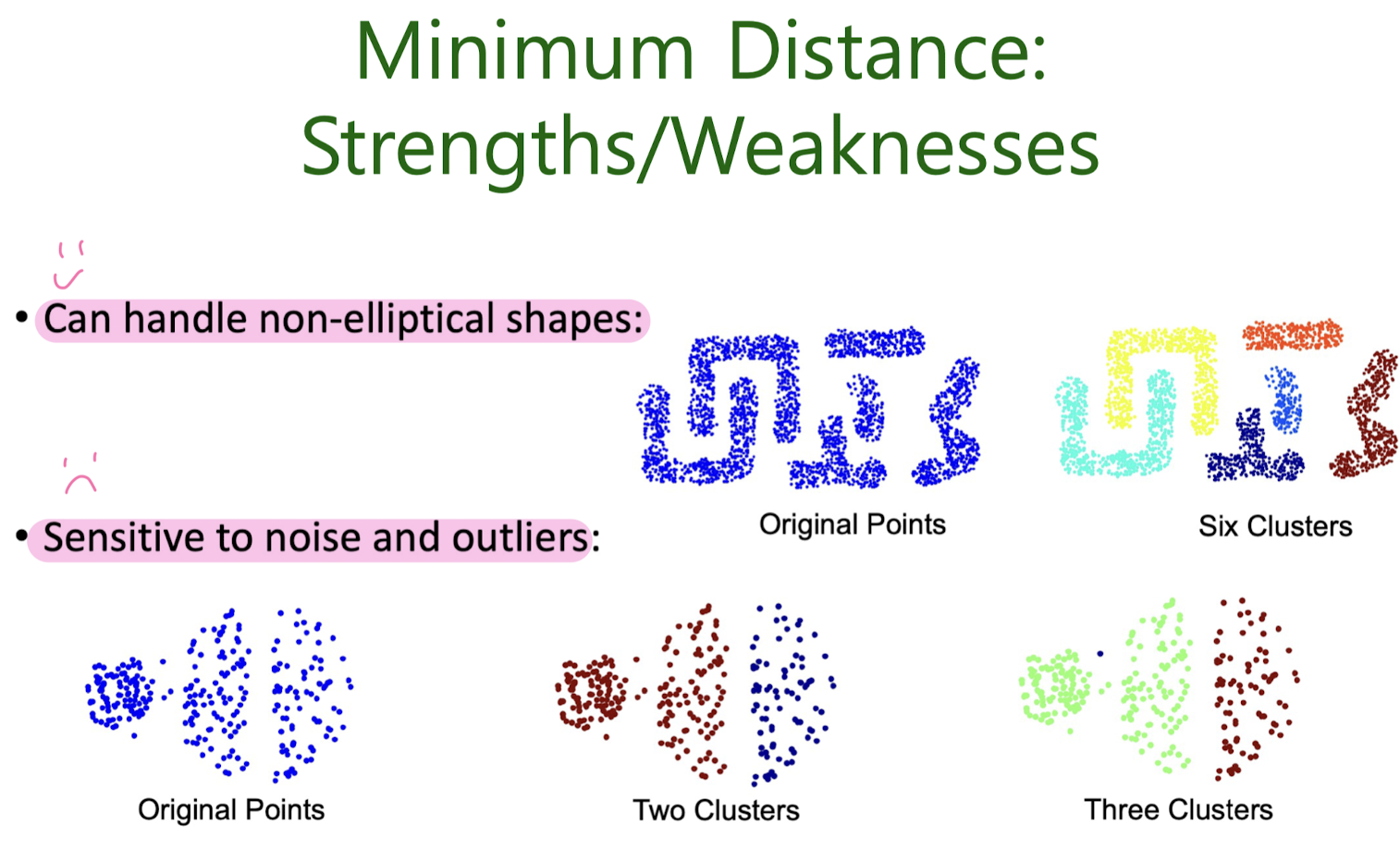
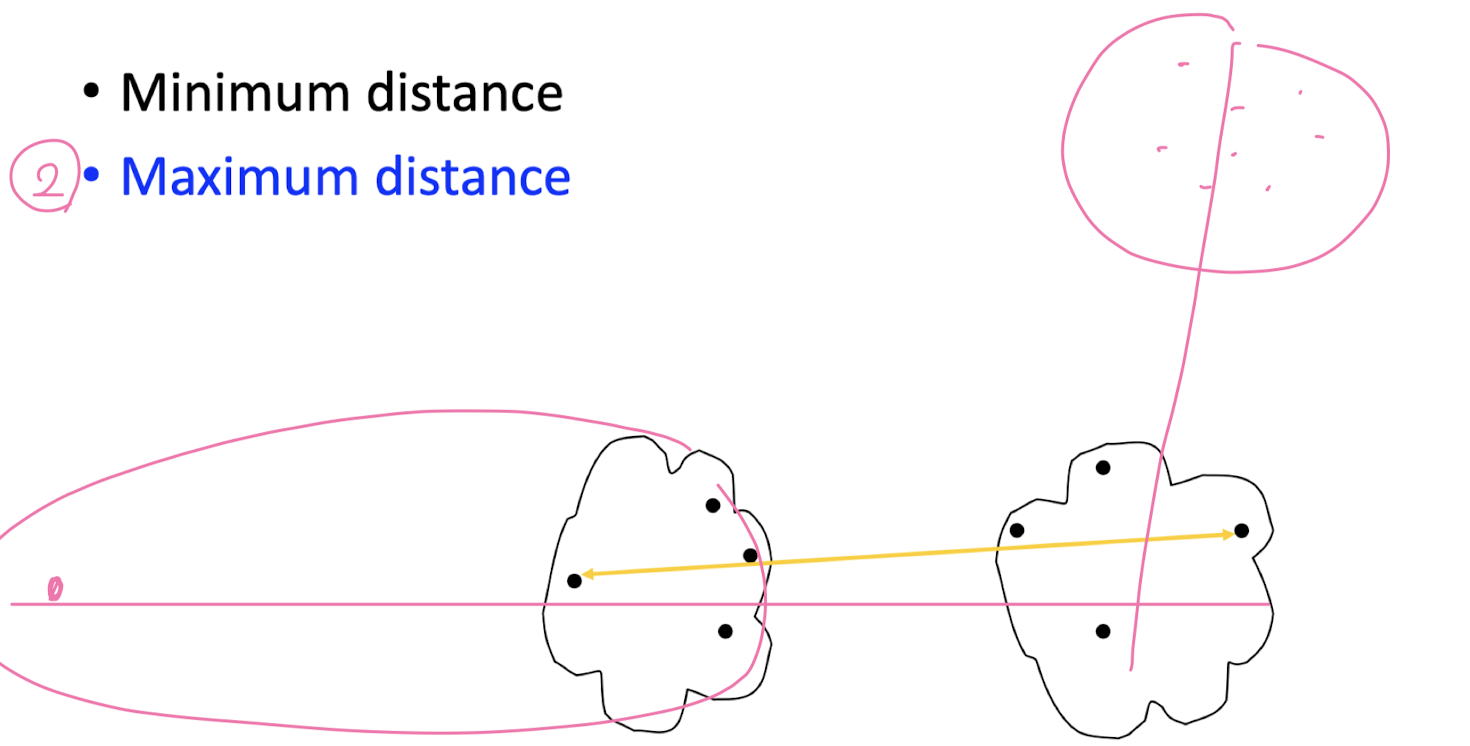
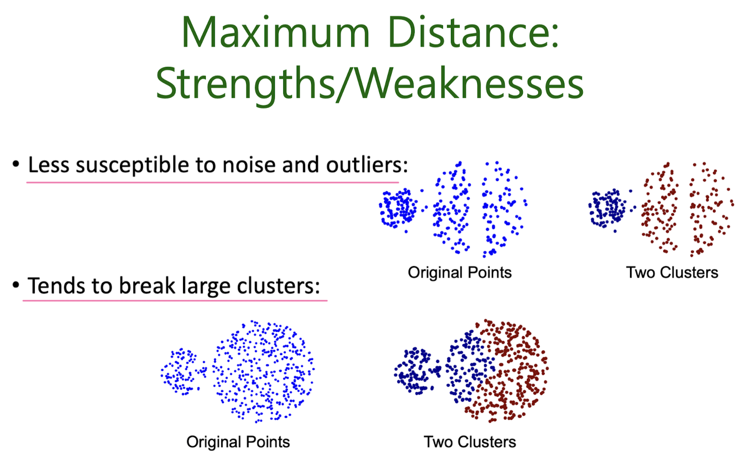
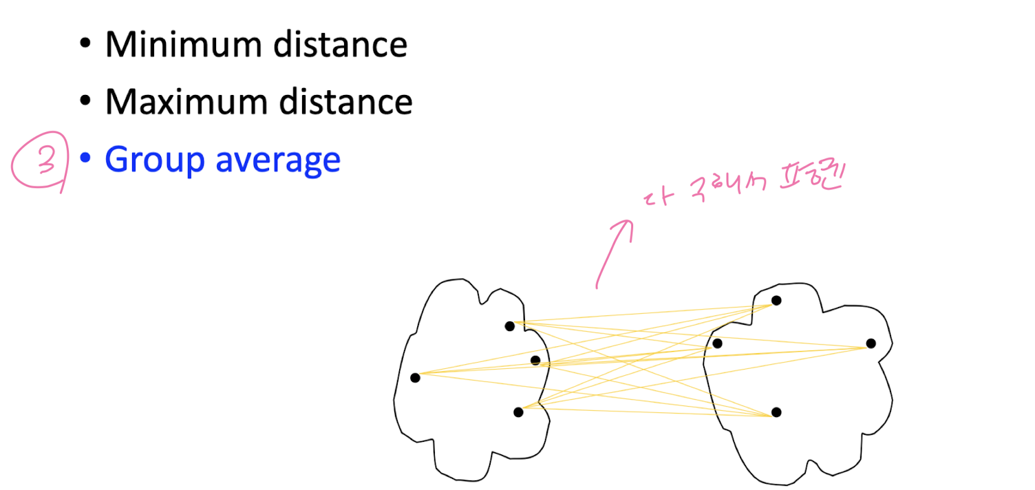
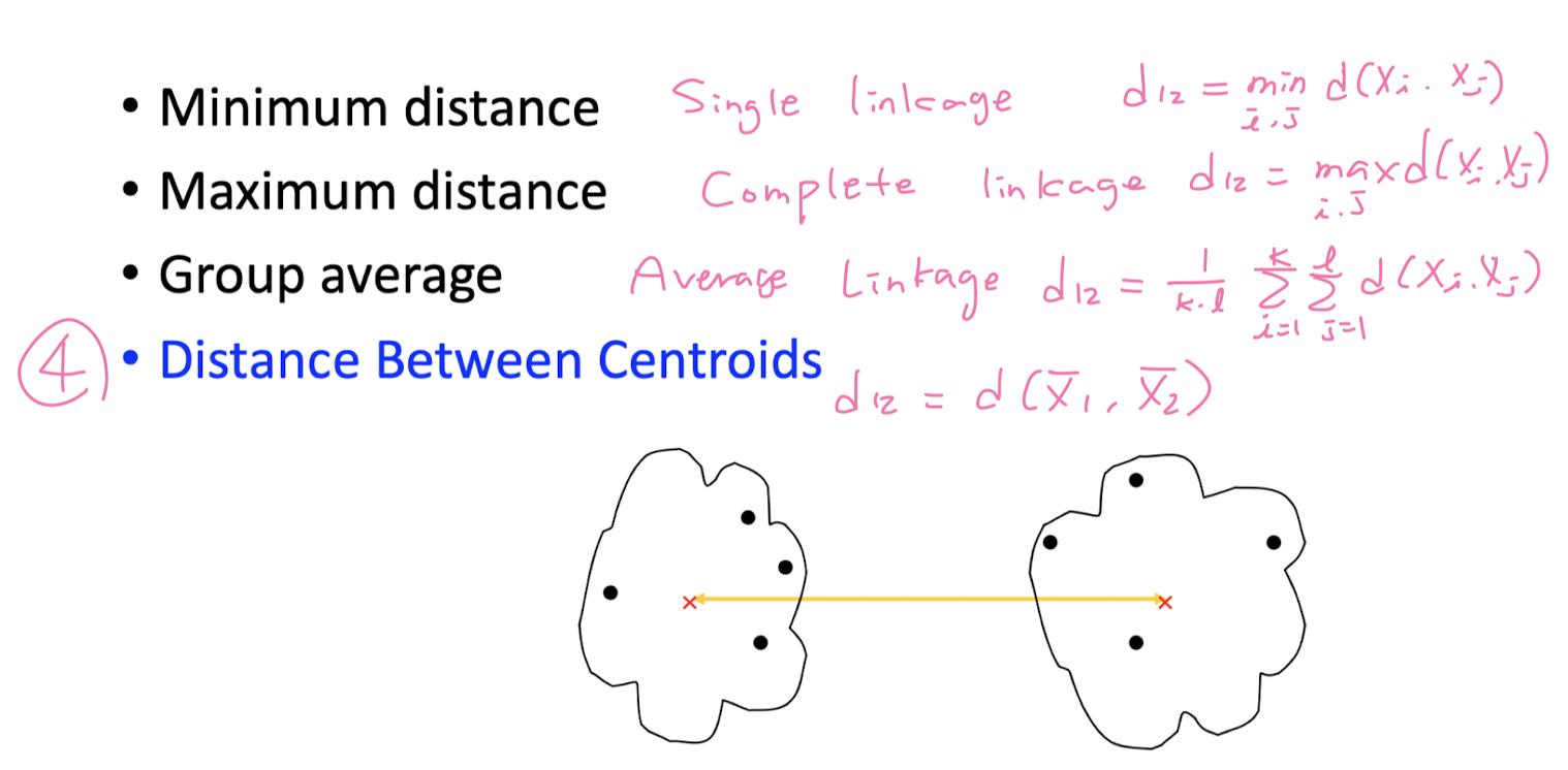
How to measure inter- cluster distance?
Divisive
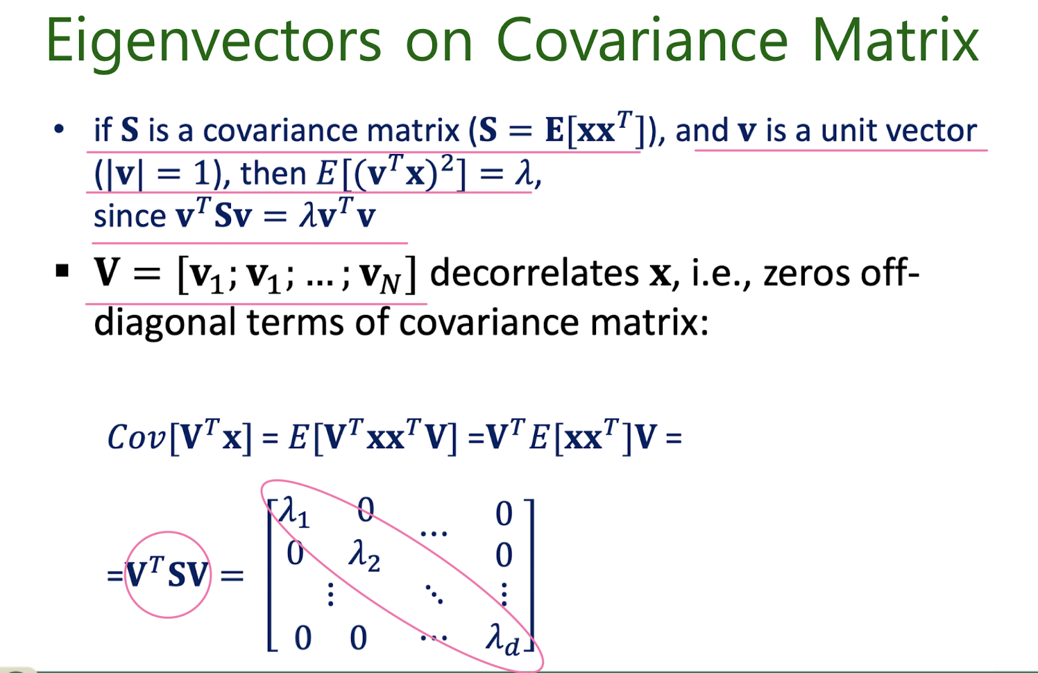
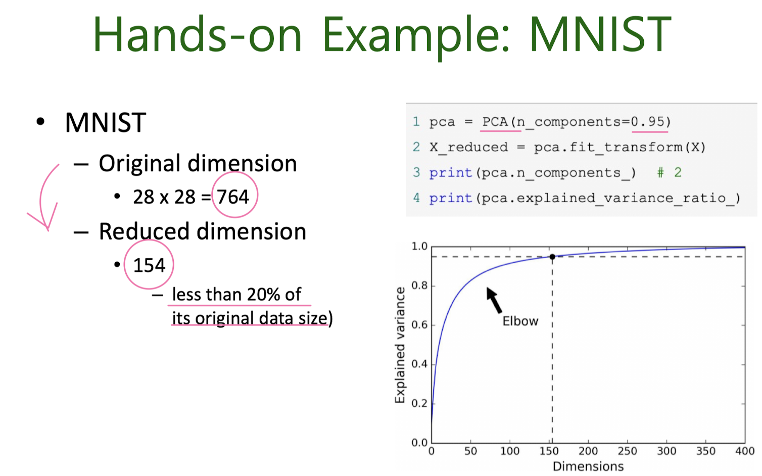
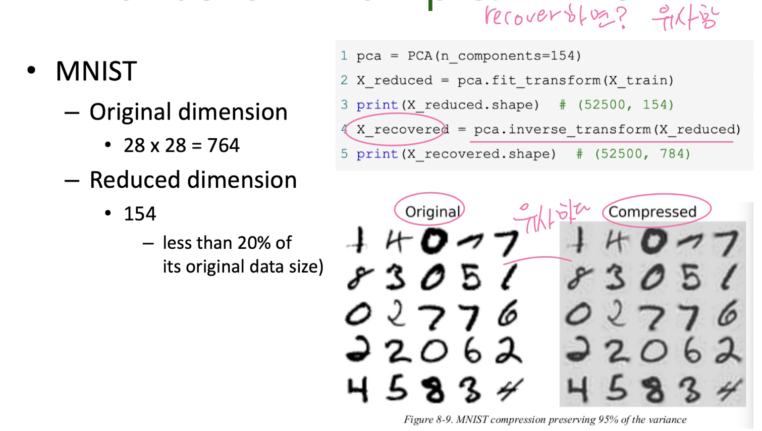
7. Unsupervised learning: Dimension Reduction
Motivation: Dimension Reduction
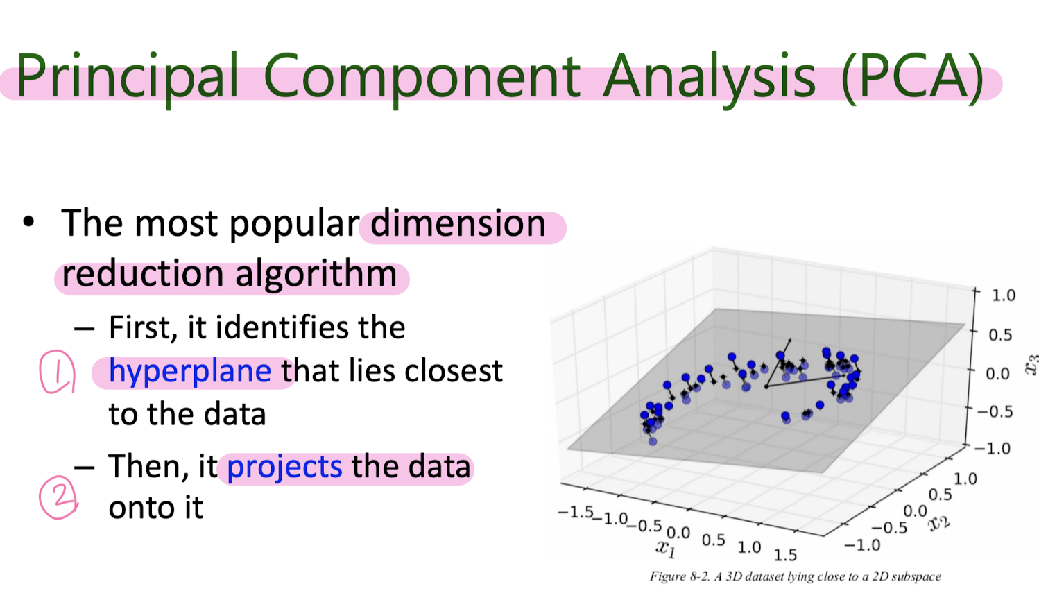
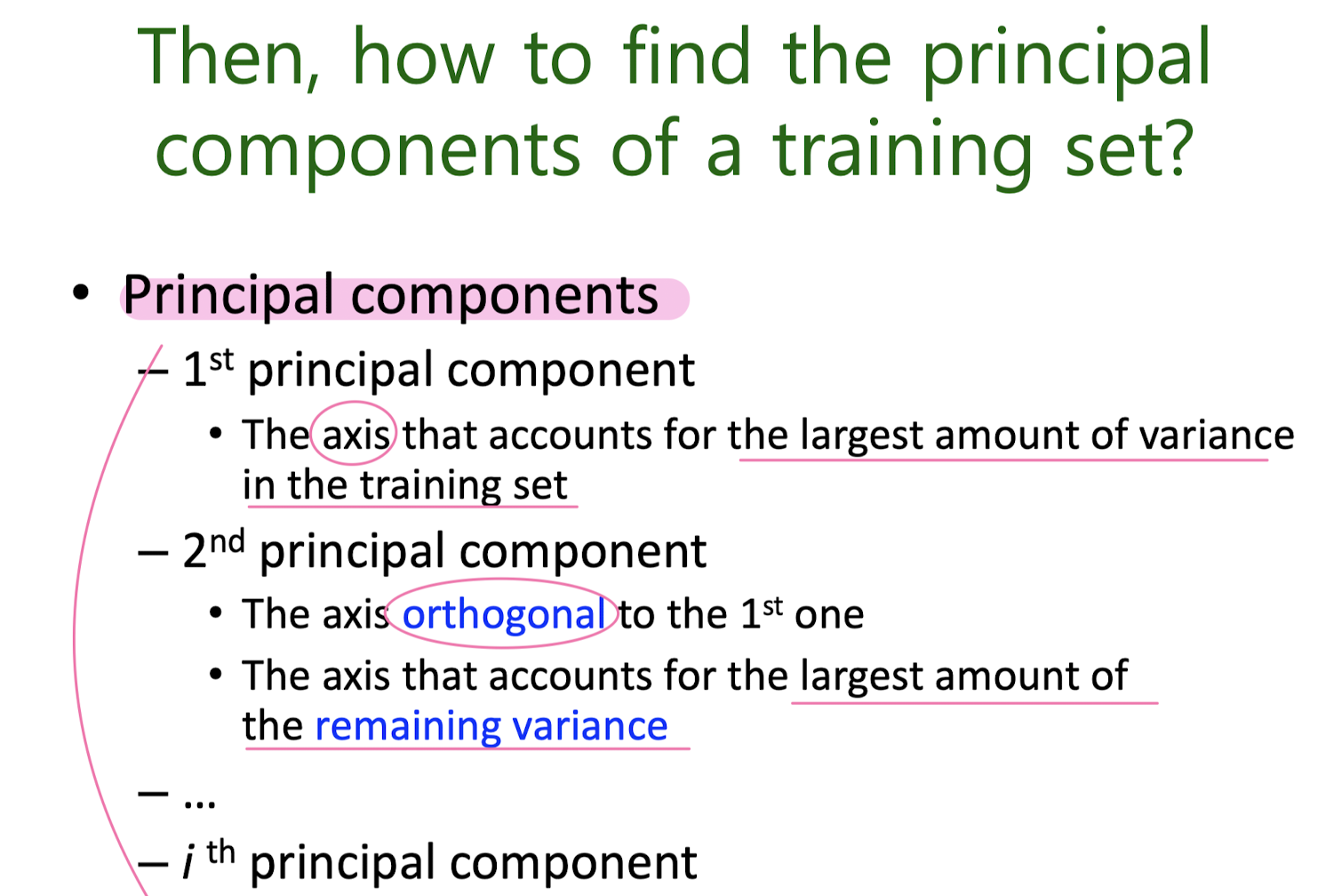
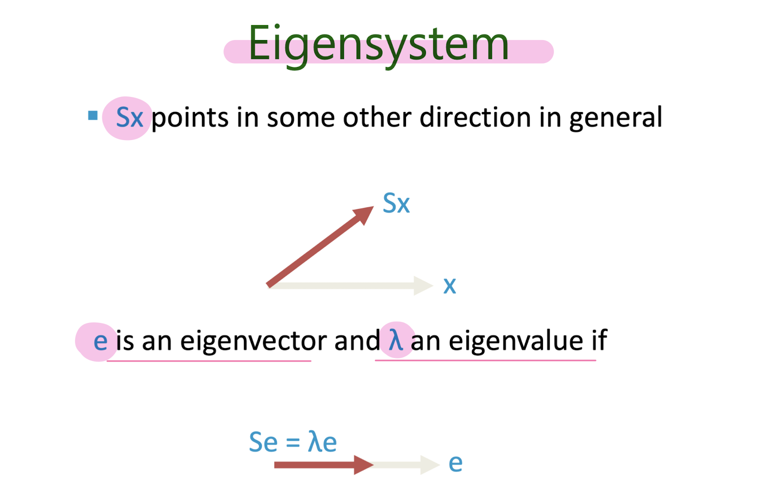
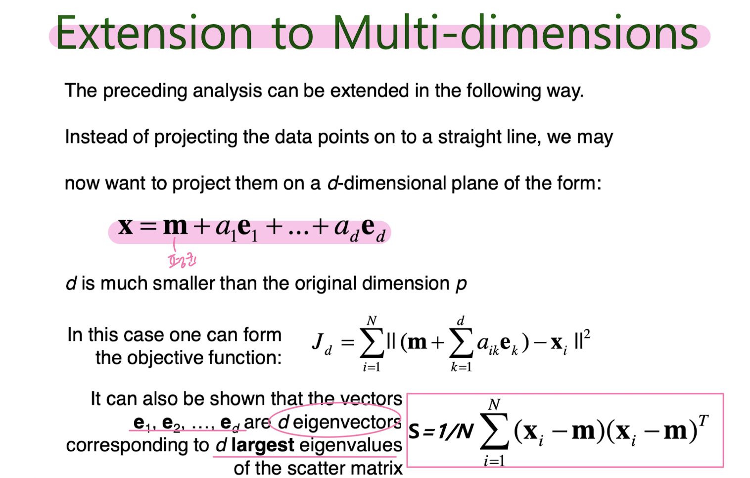
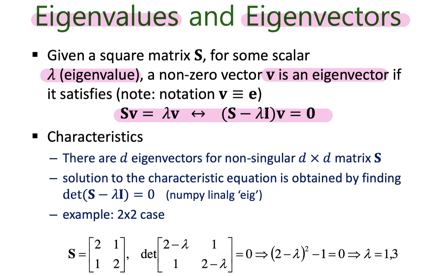
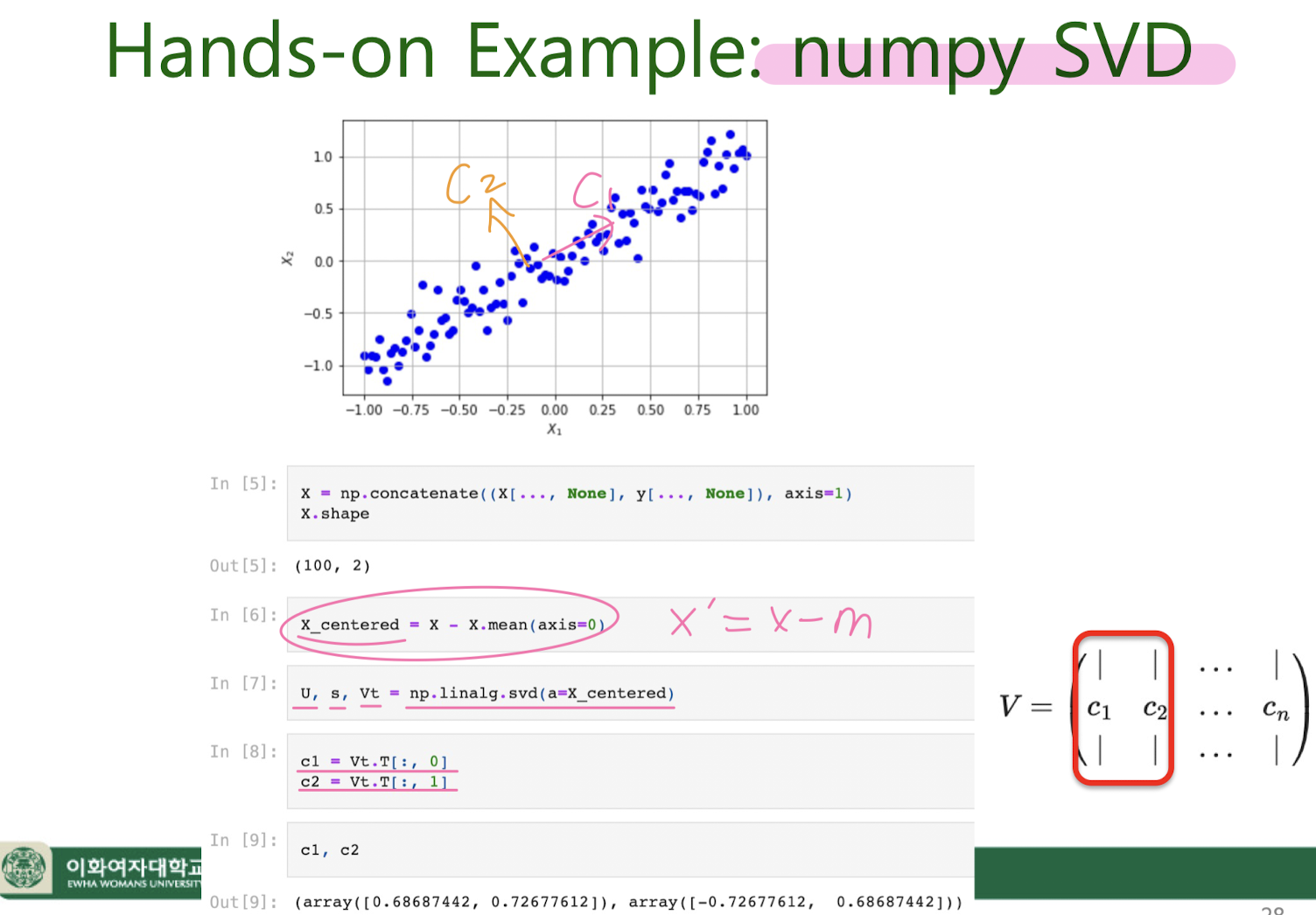
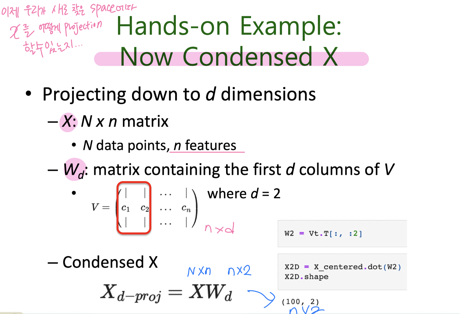
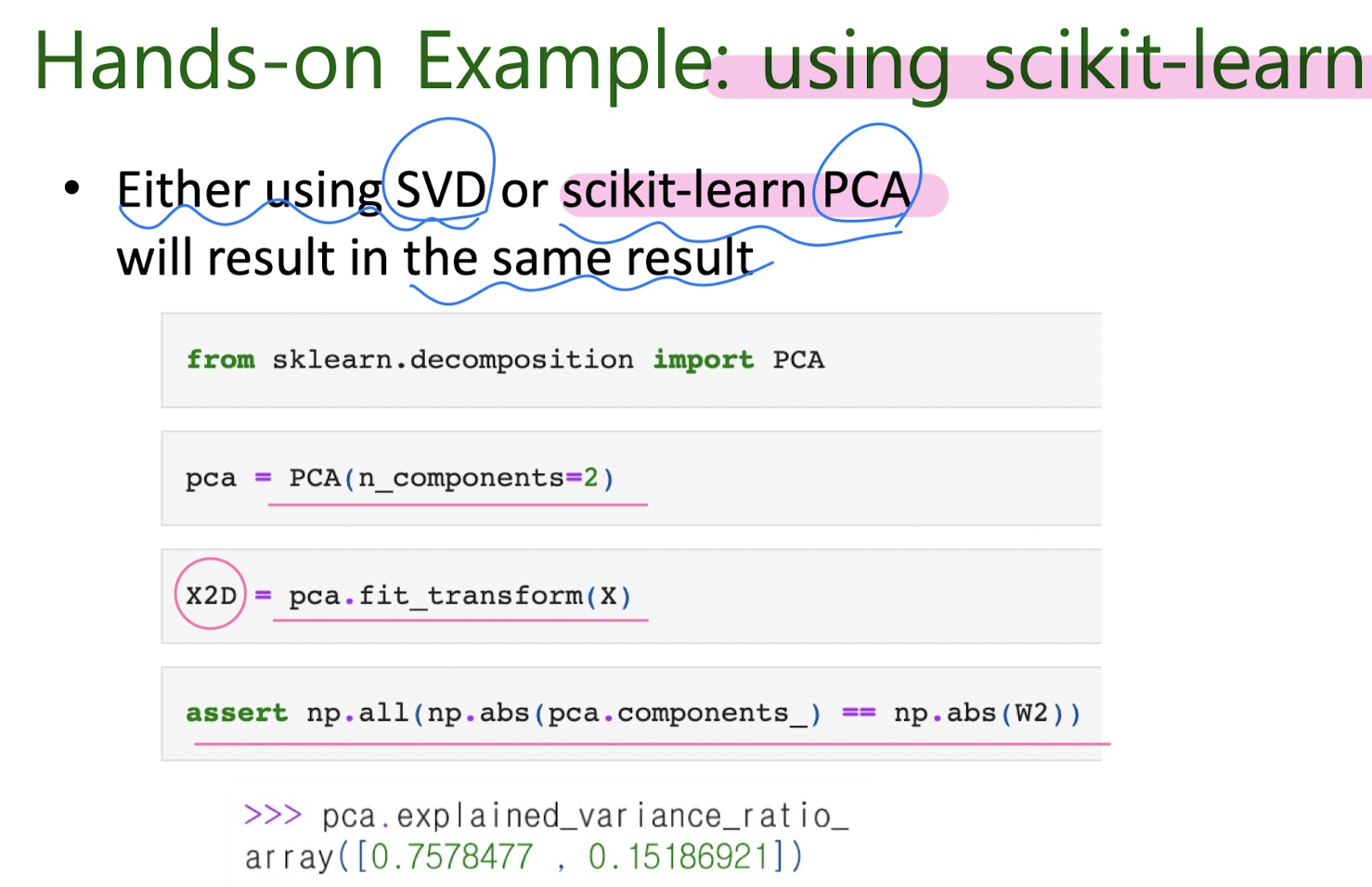
Principal Component Analysis (PCA)

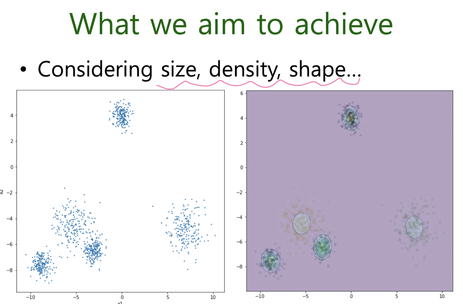
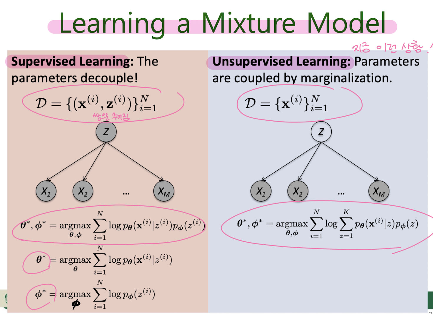
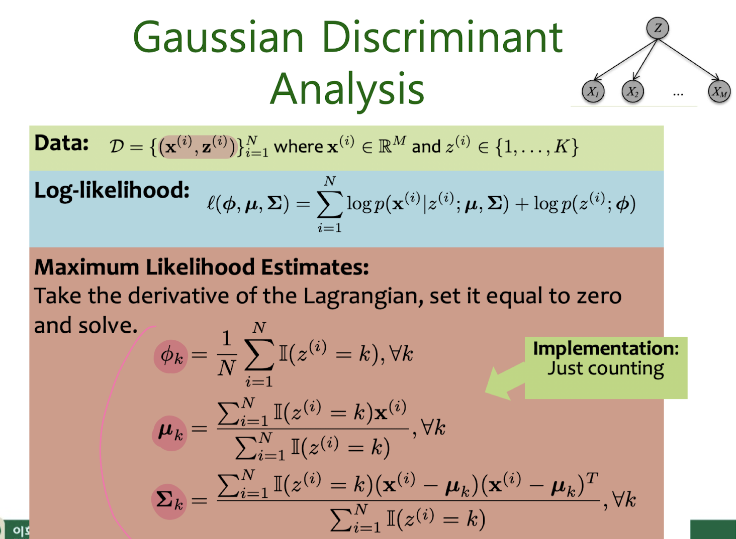
8. Unsupervised learning : GMM
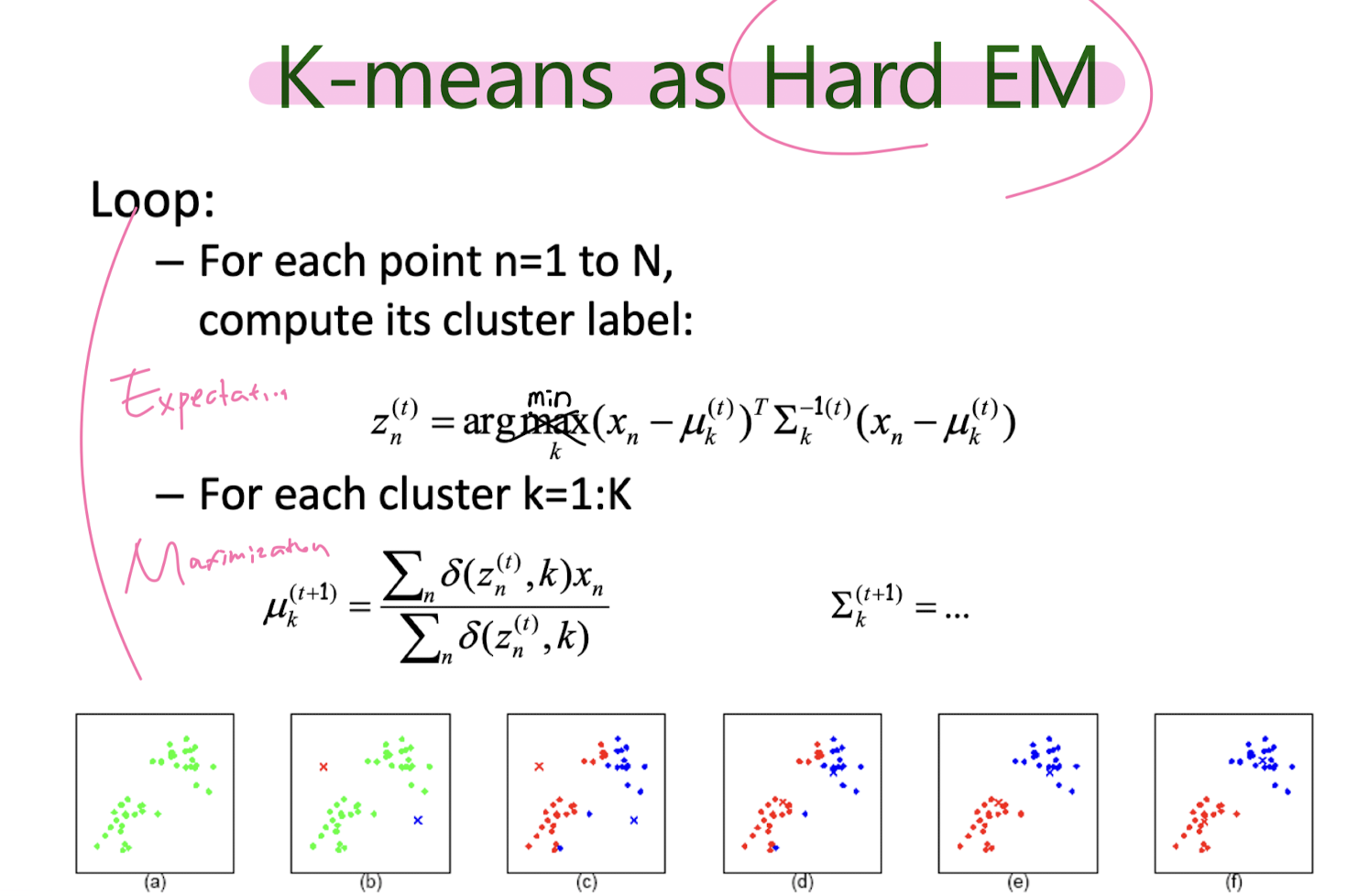
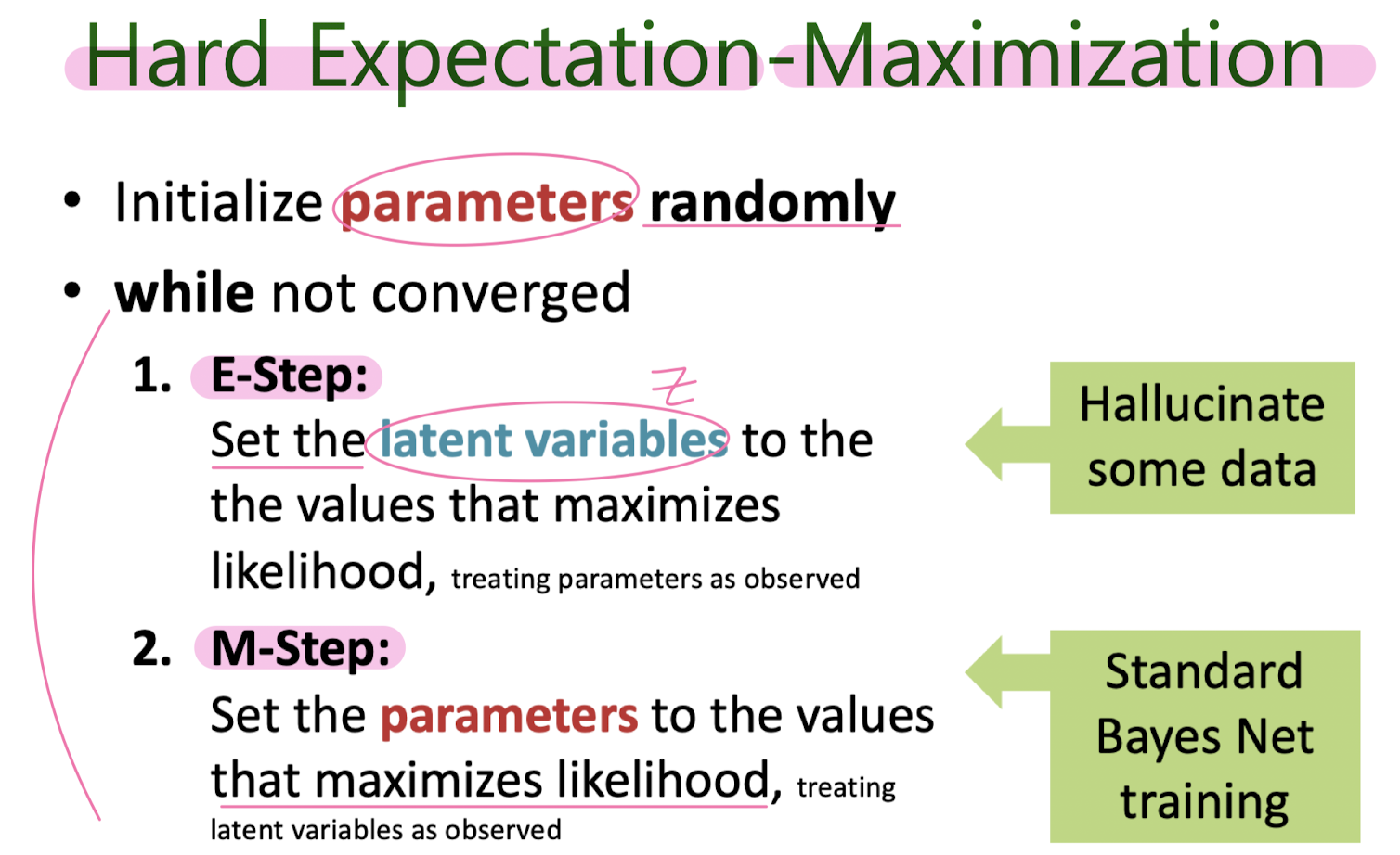
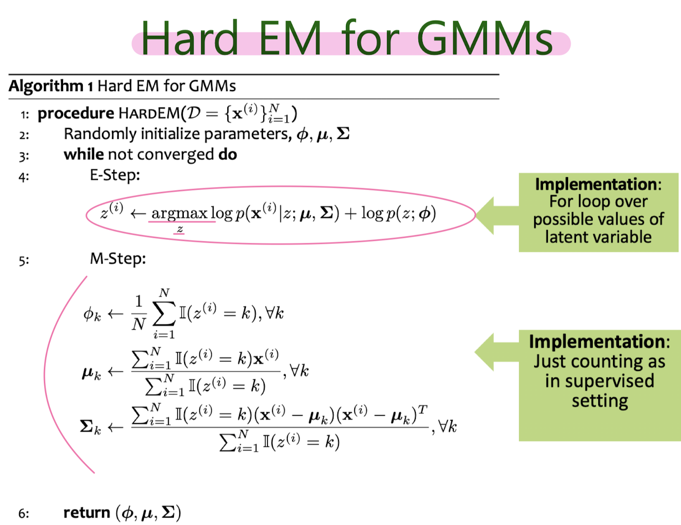
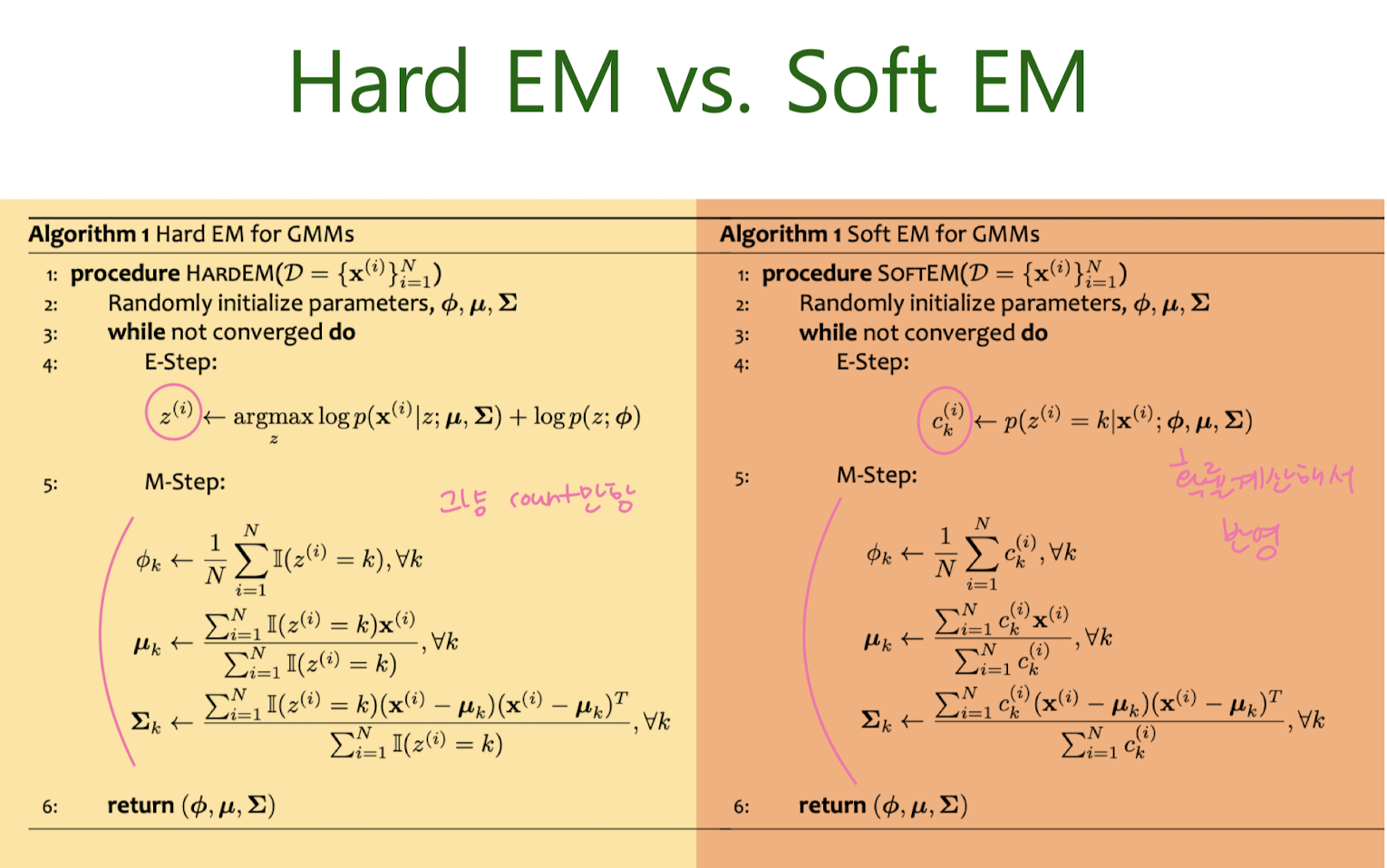
Hard EM for MM (K-means clustering)
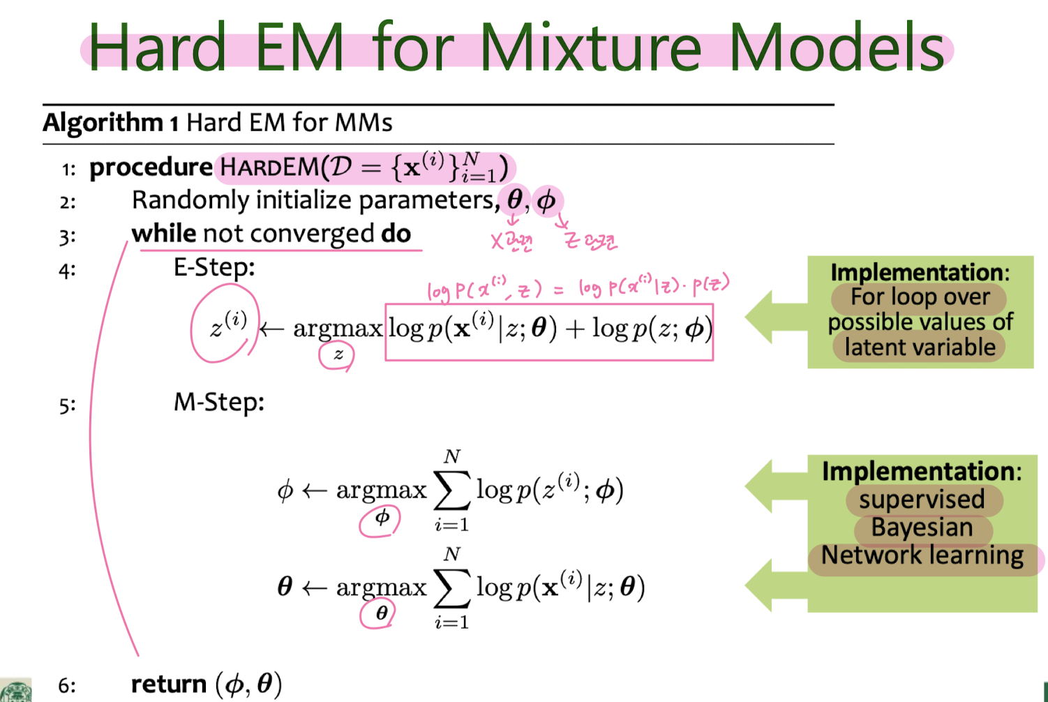
Hard EM for GMM
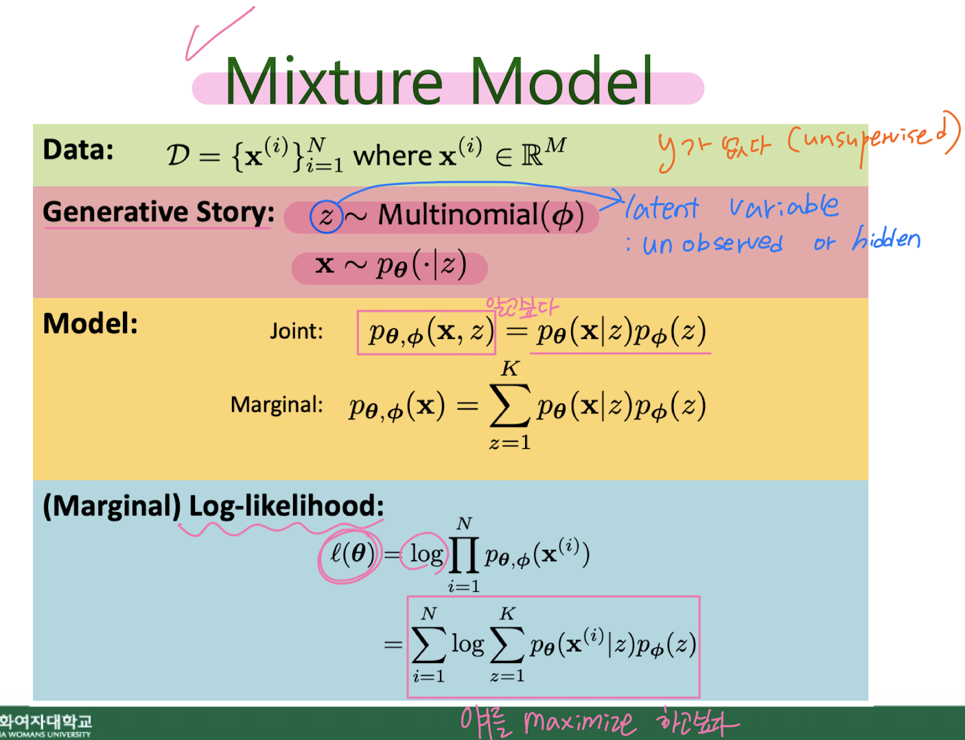
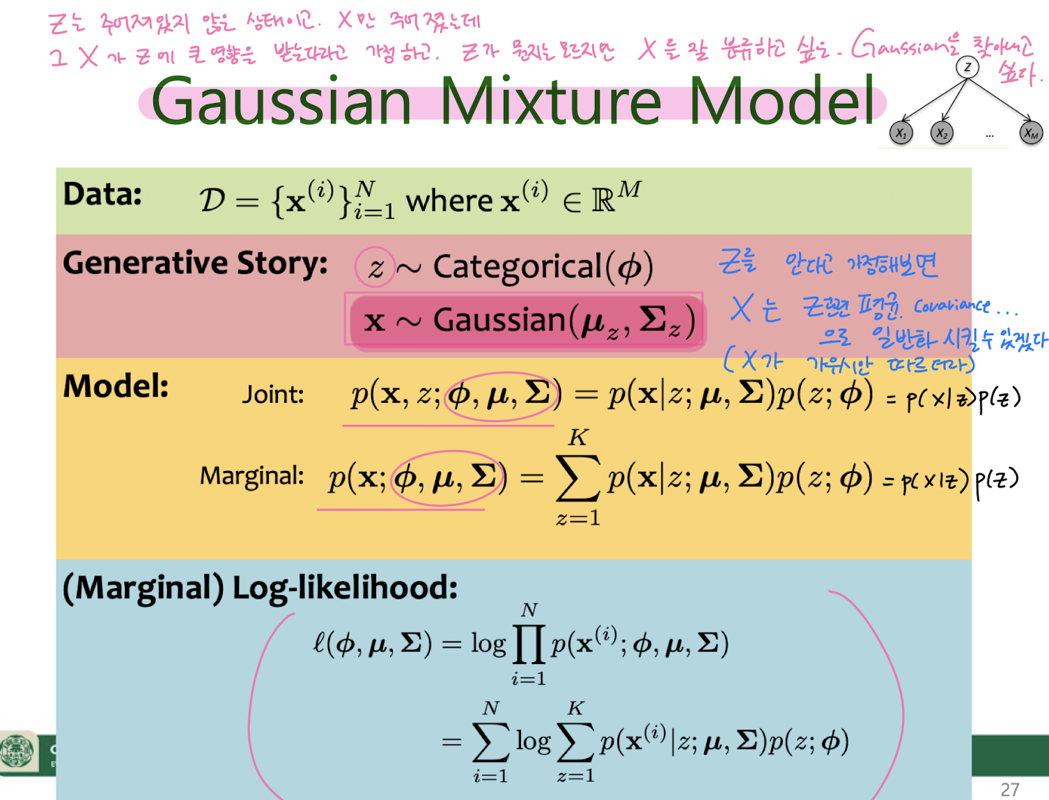
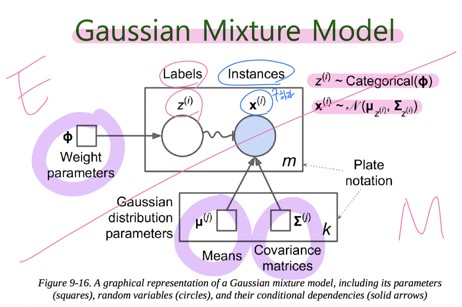
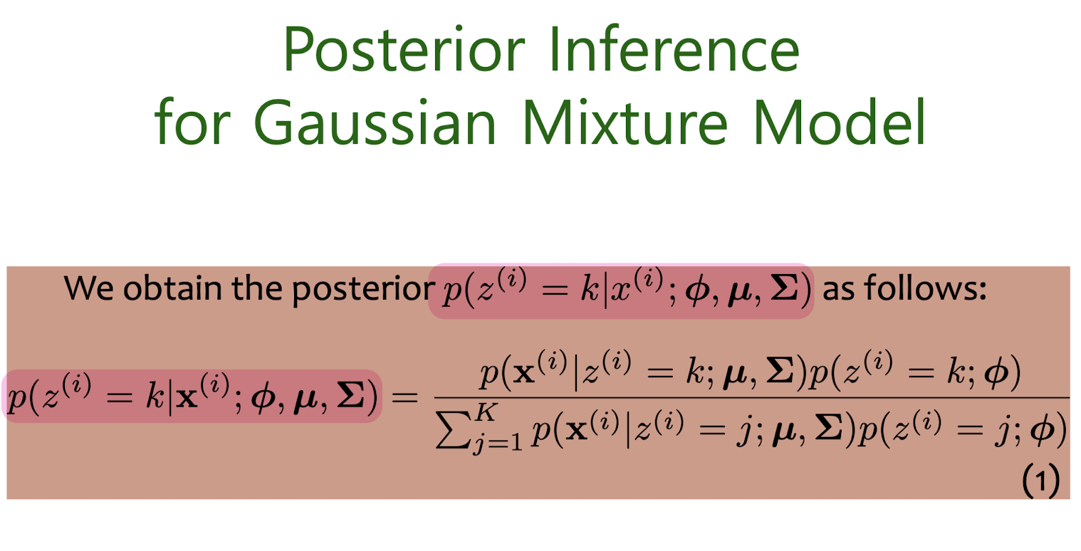
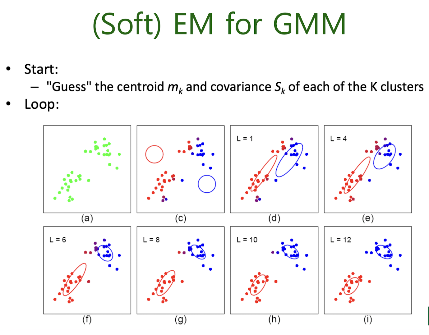
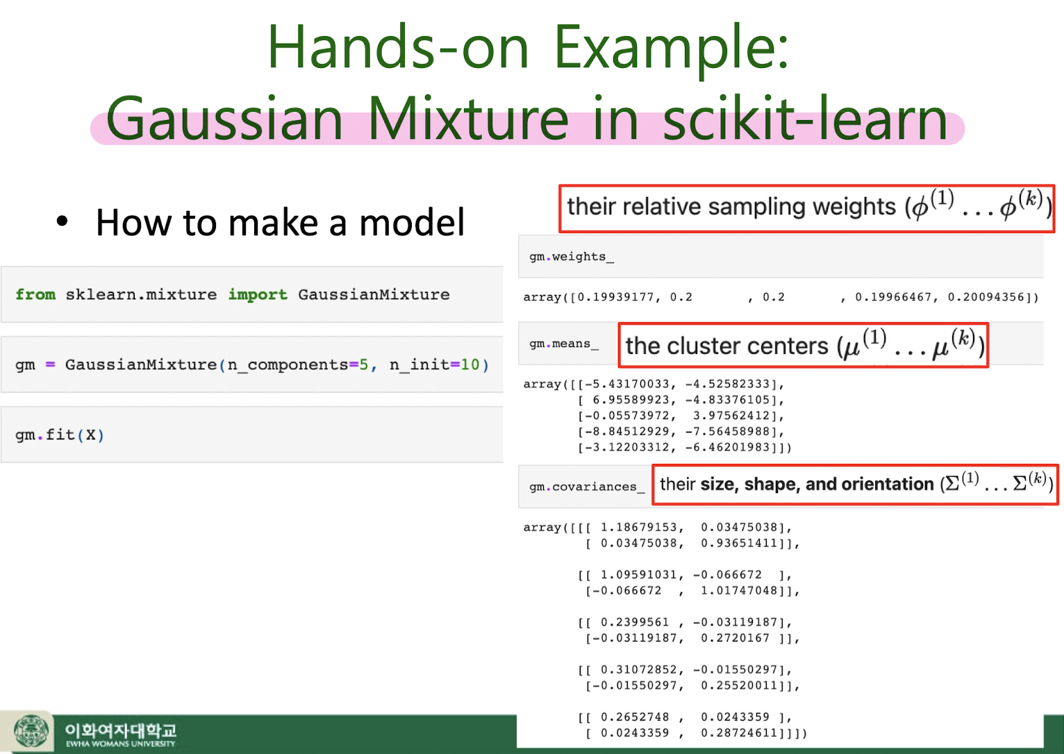
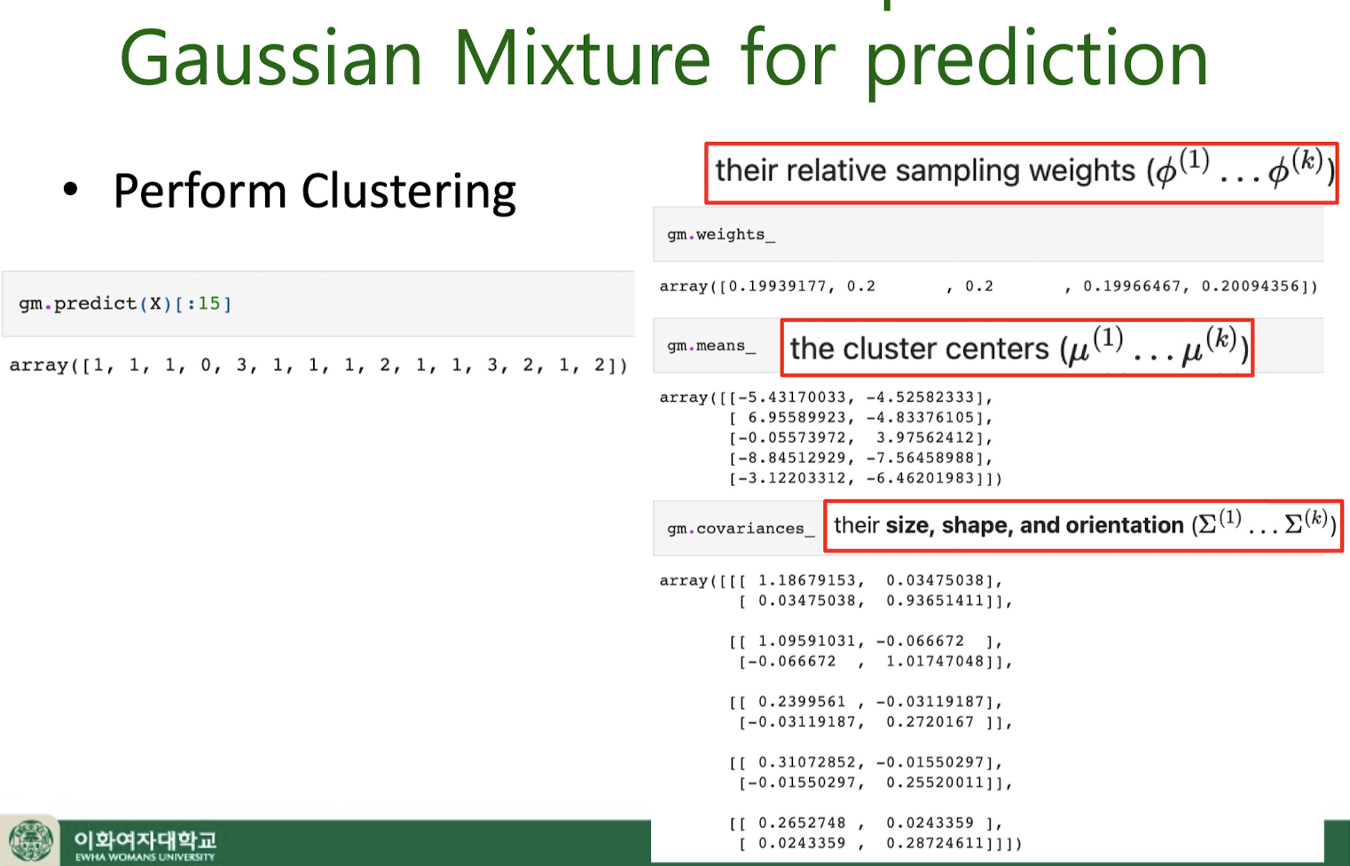
Gaussian Mixture Model (GMM)
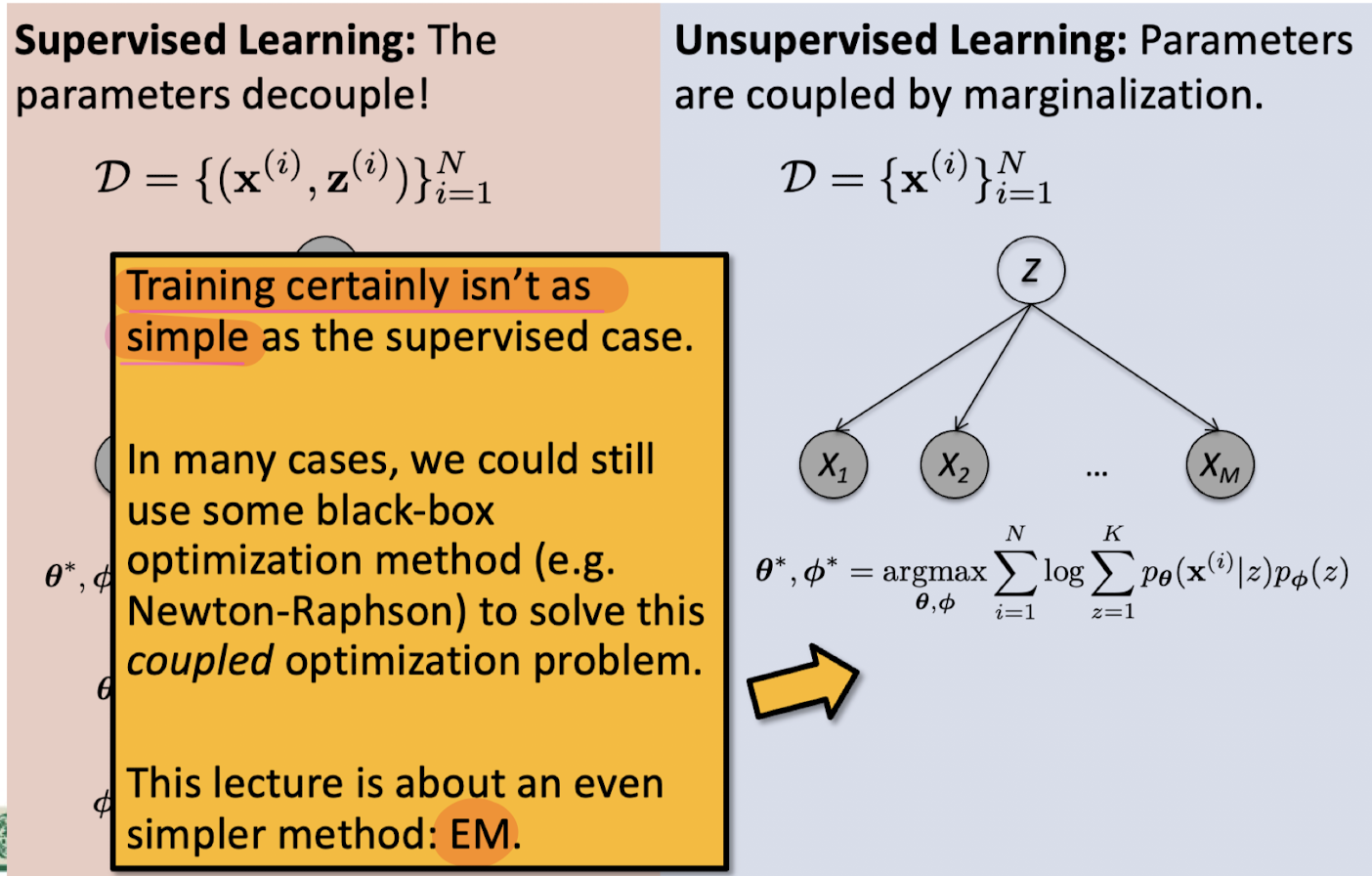
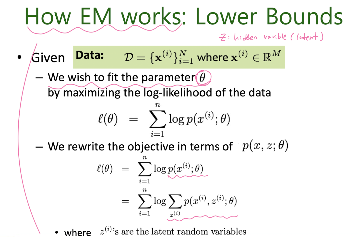
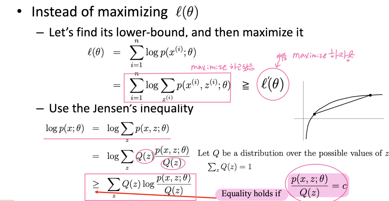
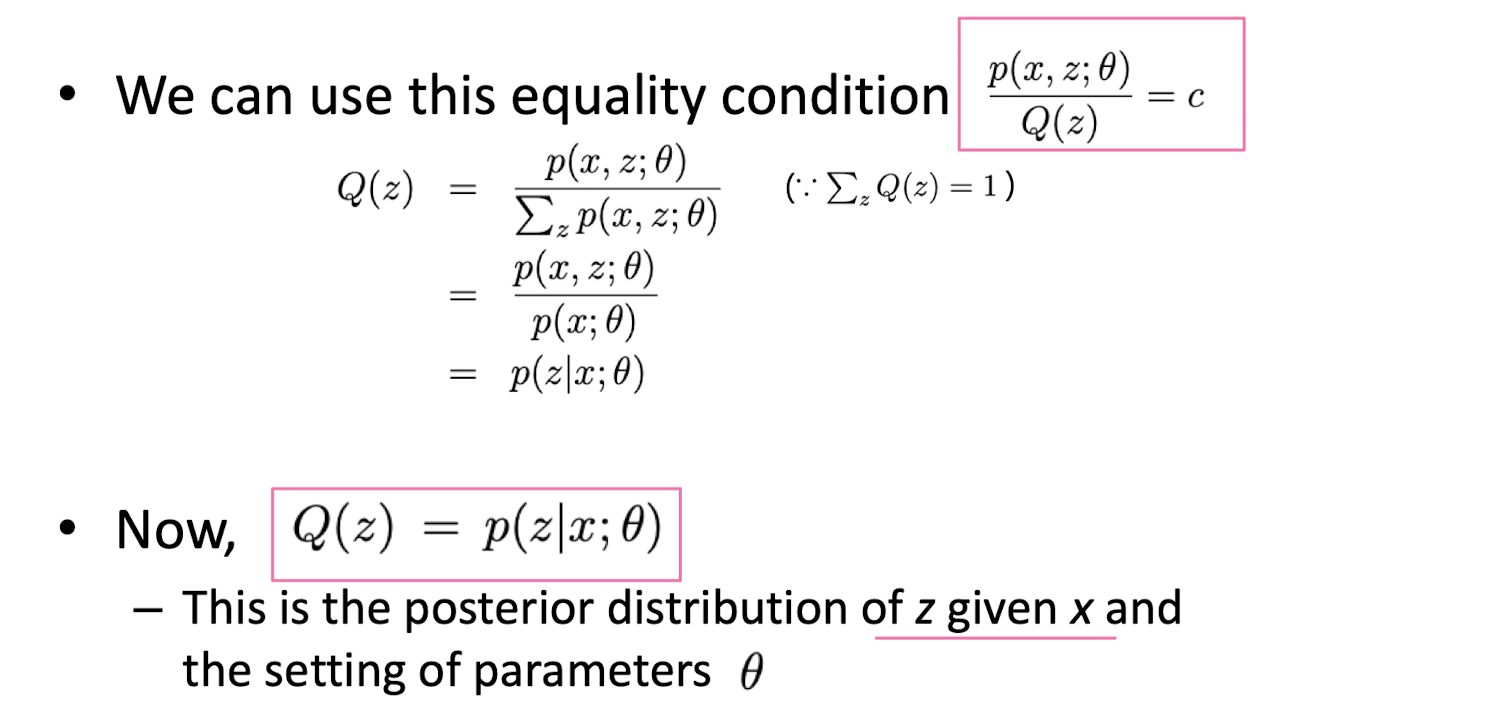
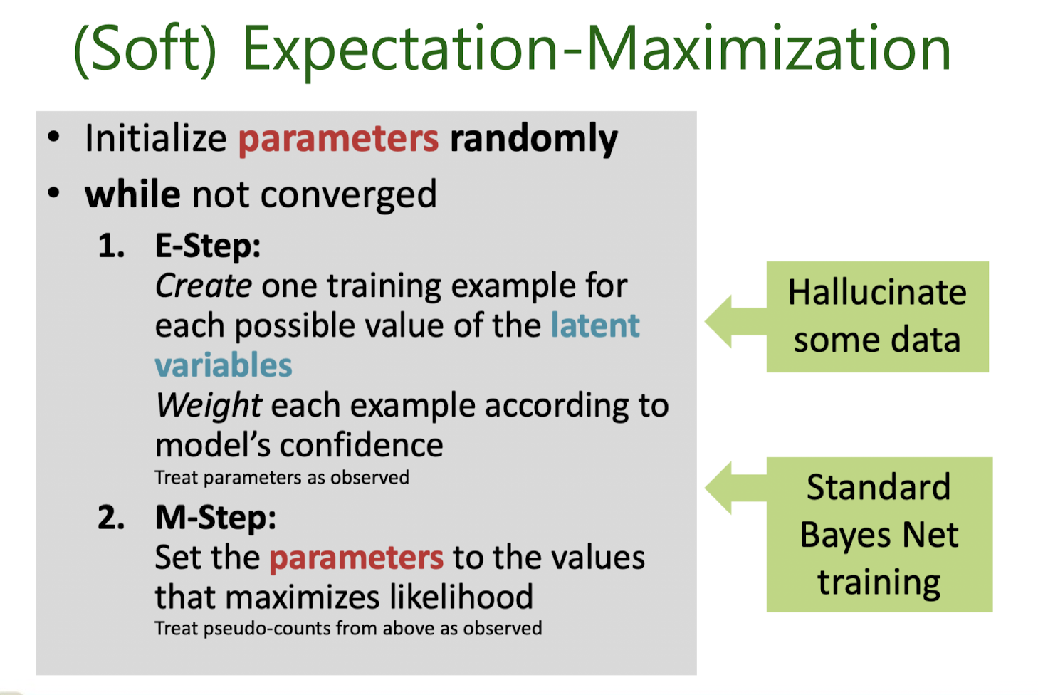
Expectation-Maximization (EM) Algorithm
How EM works: Lower Bound
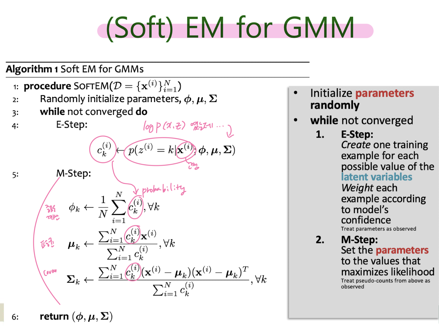
Soft EM for GMM

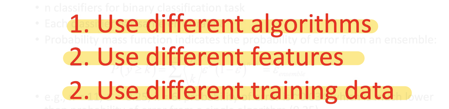
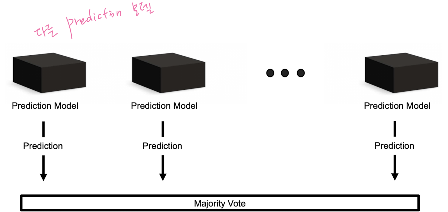
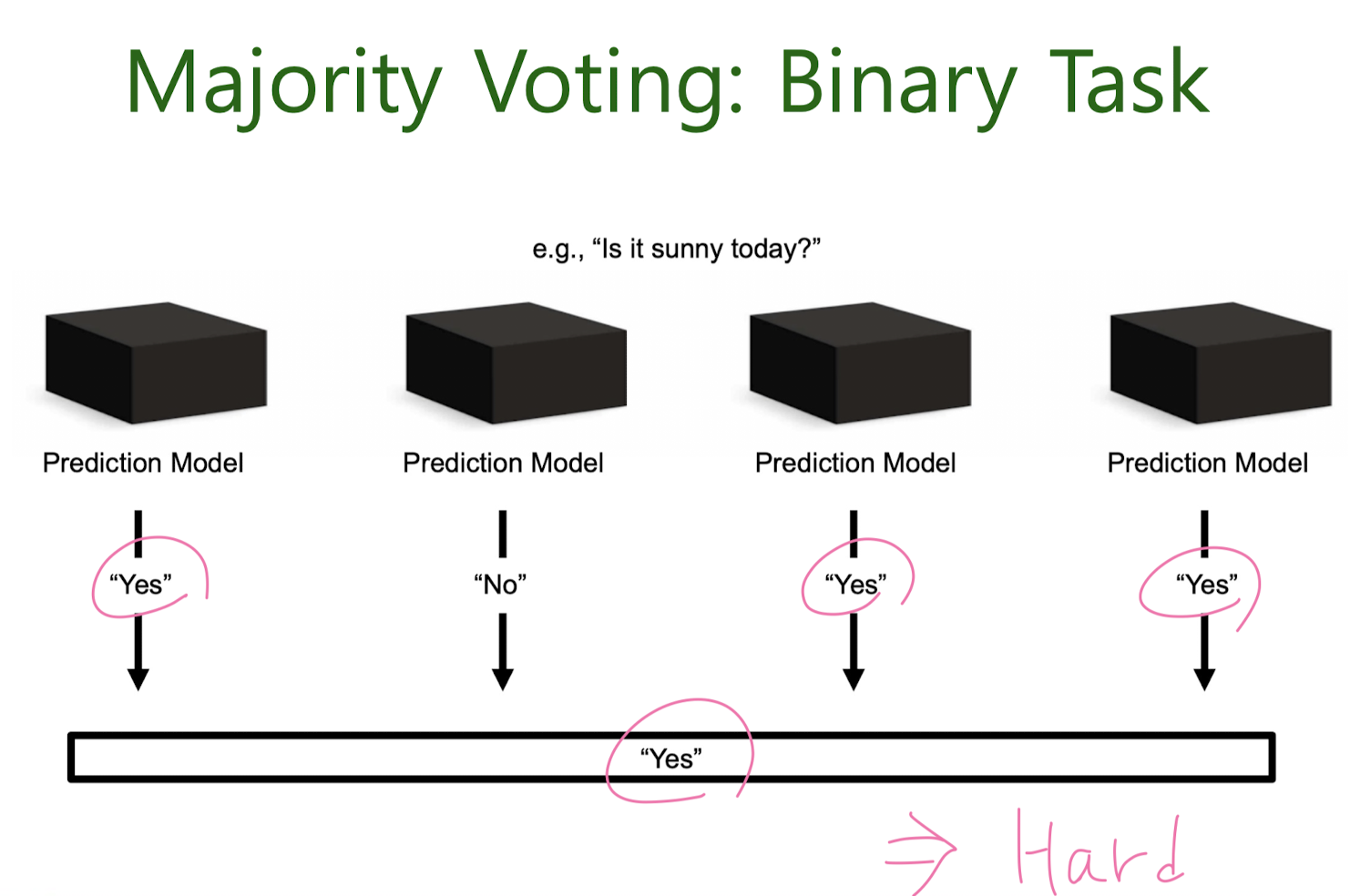
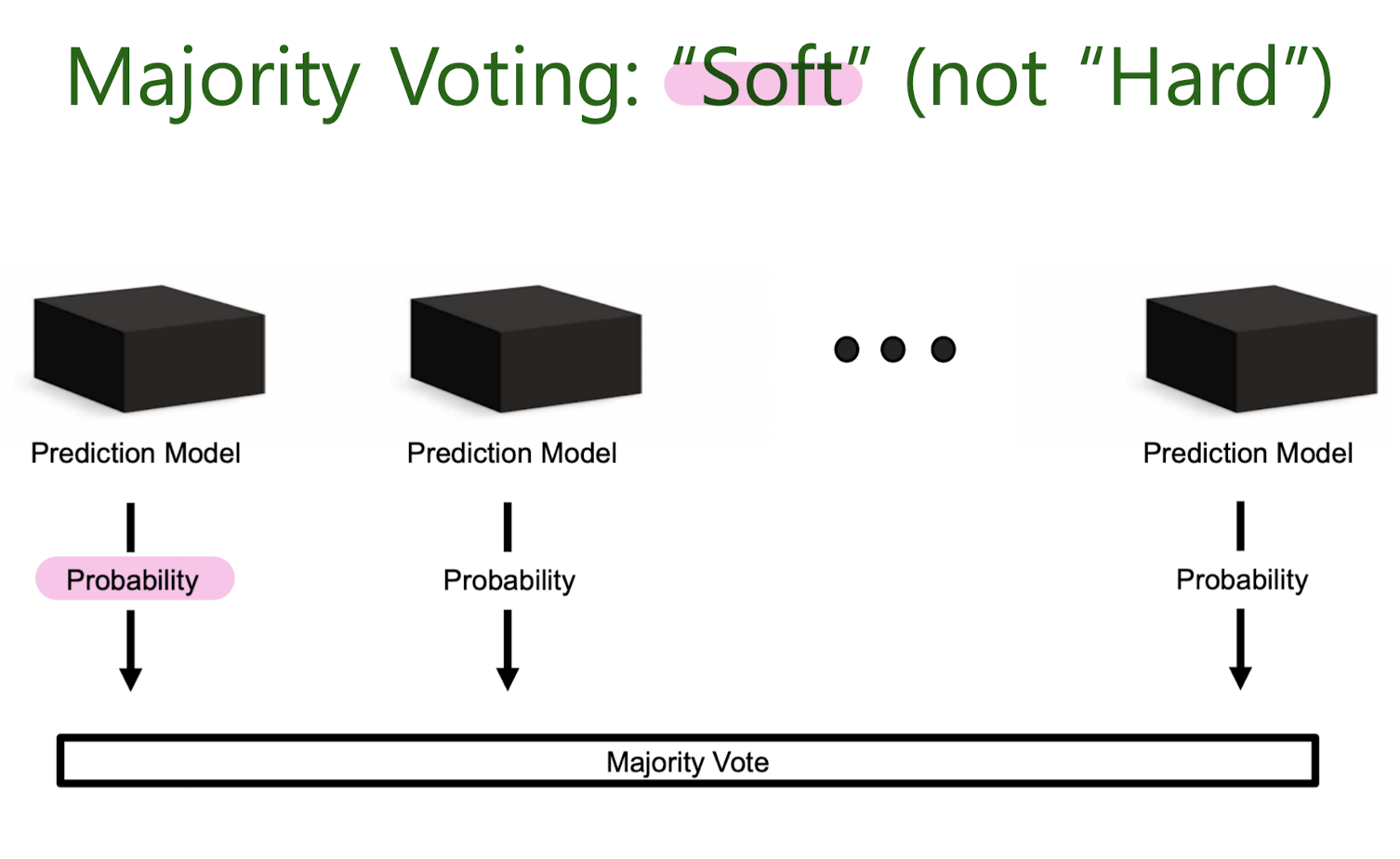
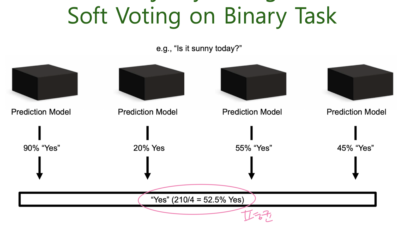
8. Ensemble Learning
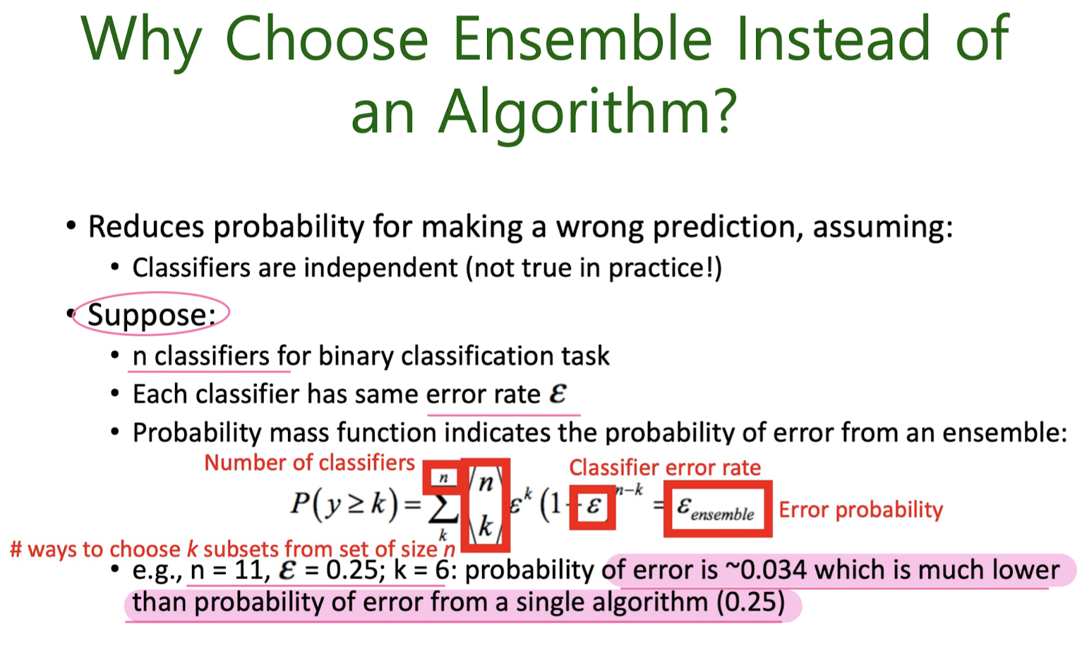
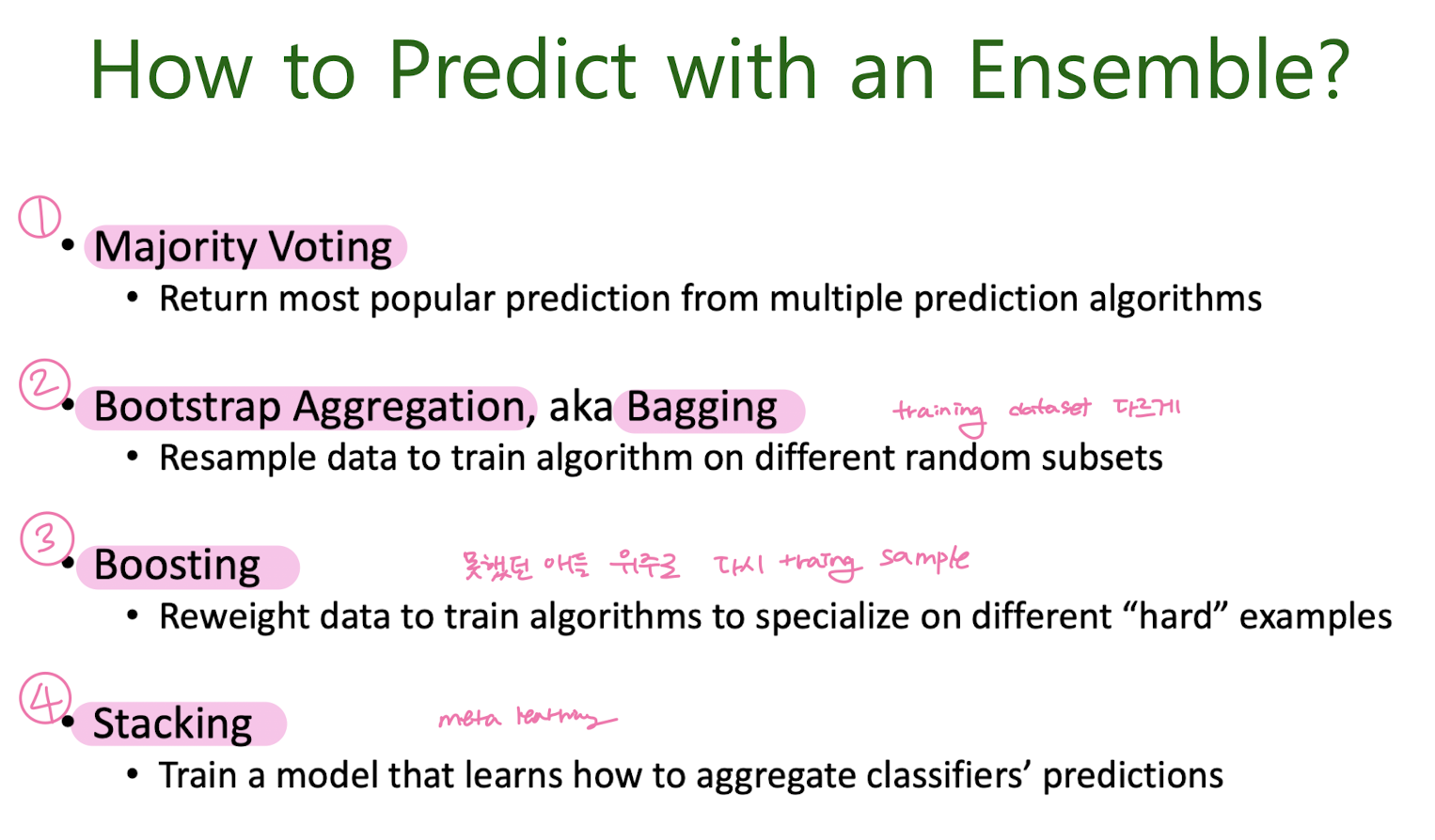
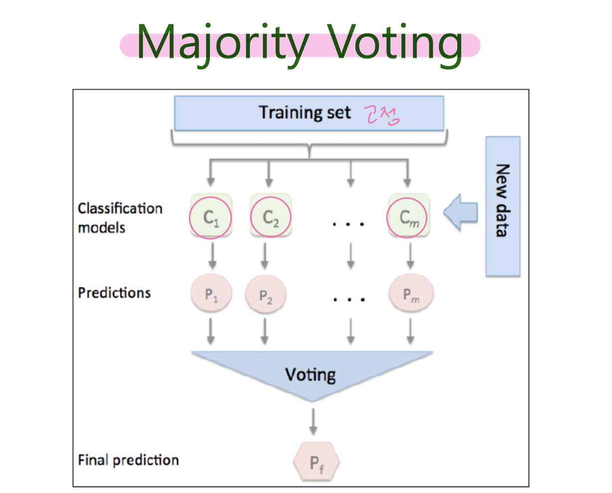
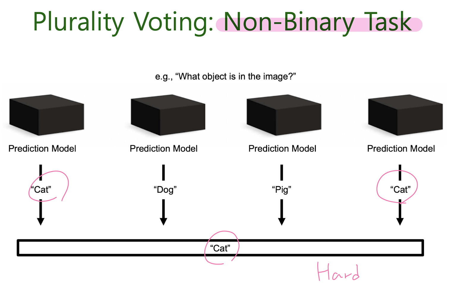
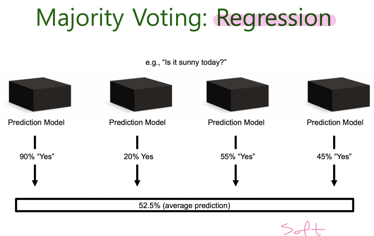
Majority Voting

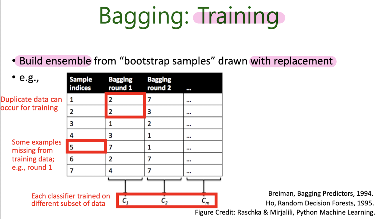
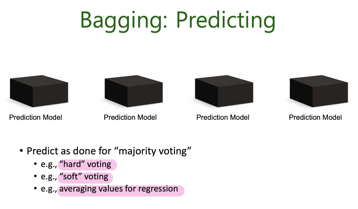
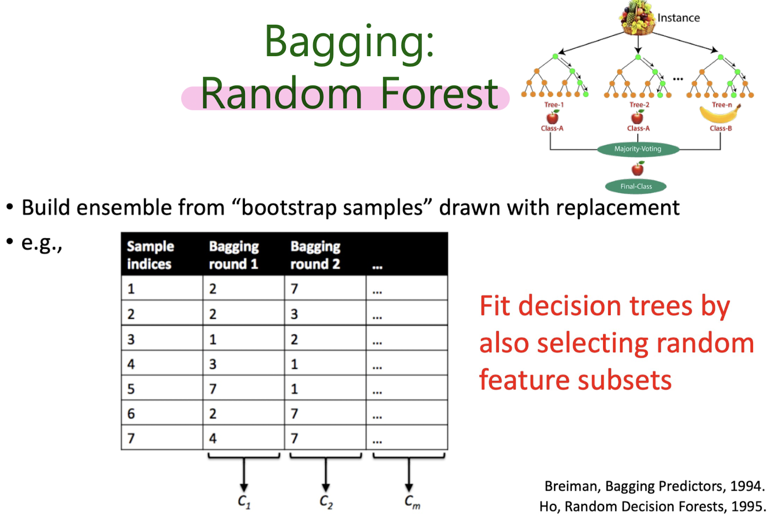
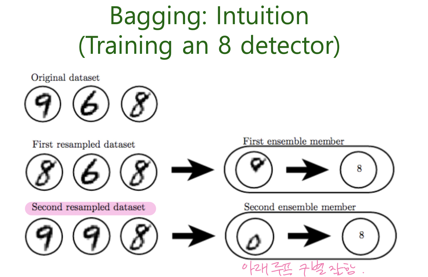
Bootstrap Aggregation, Bagging
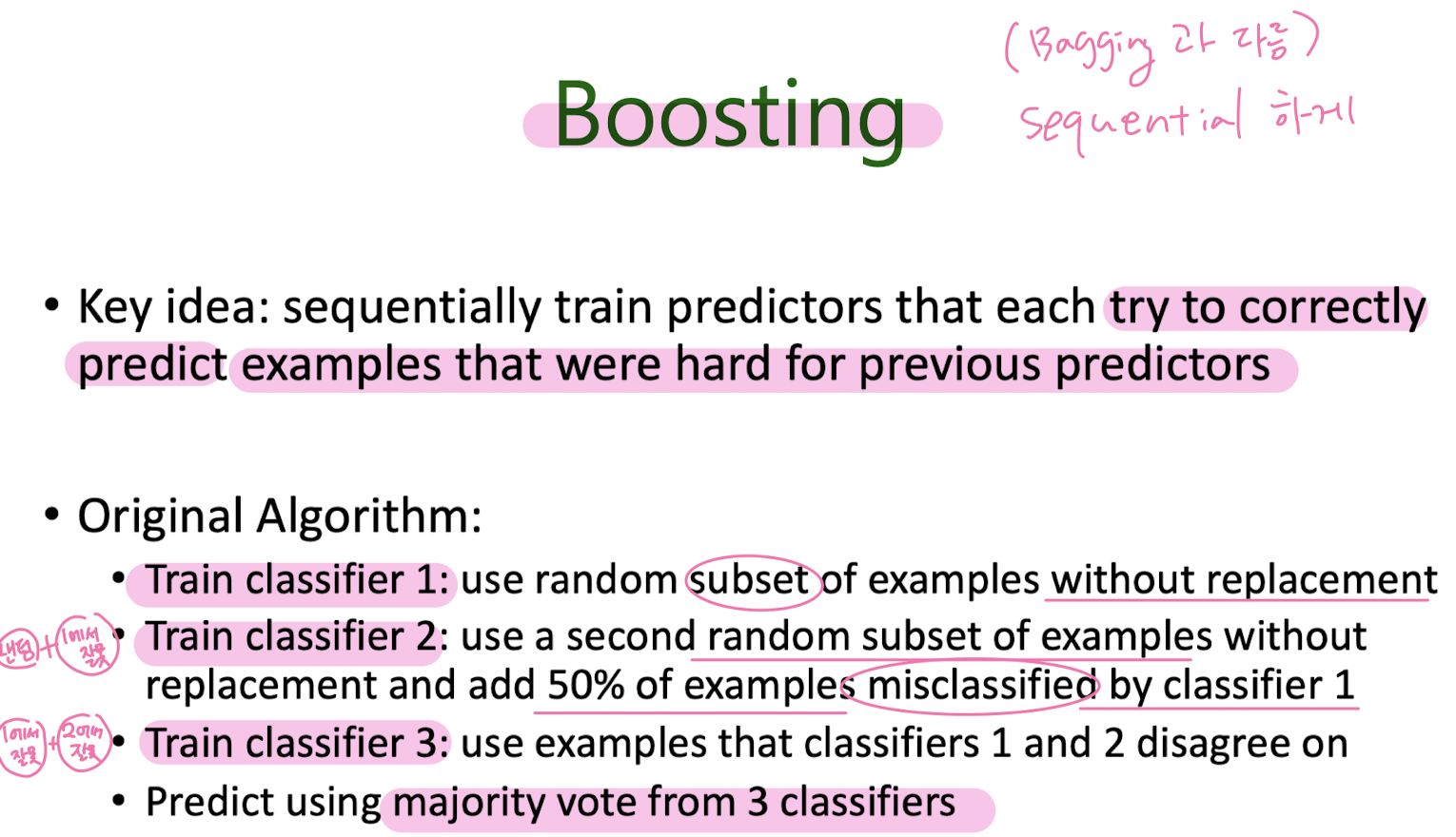
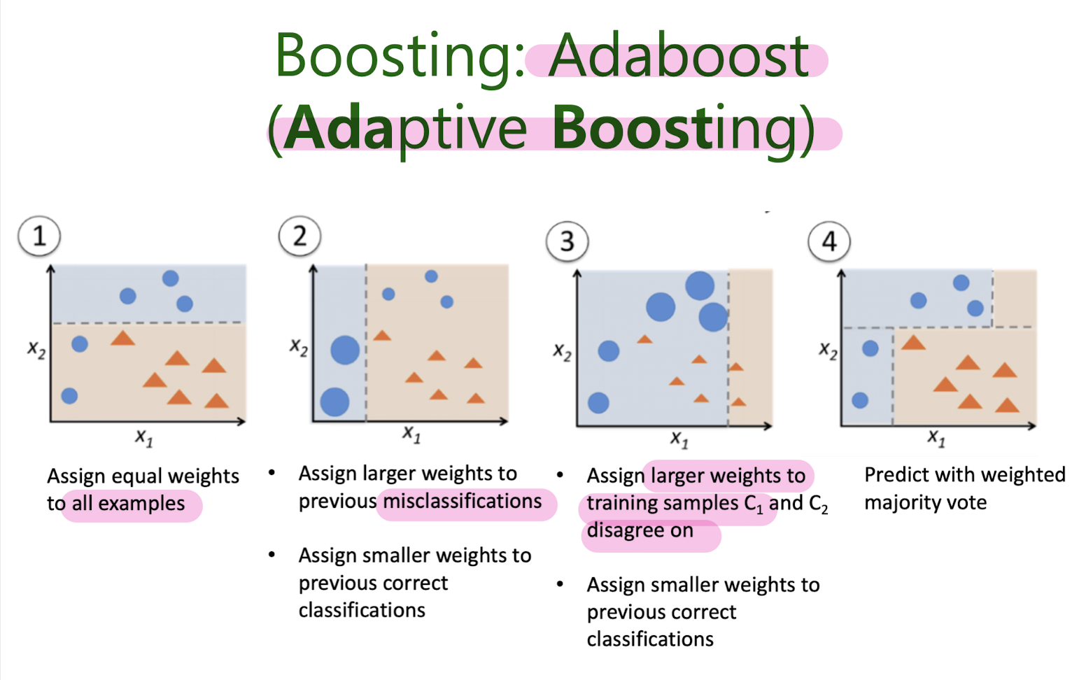
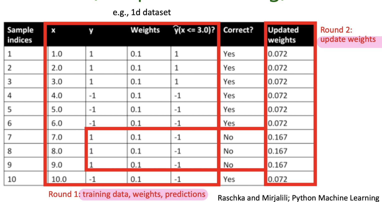
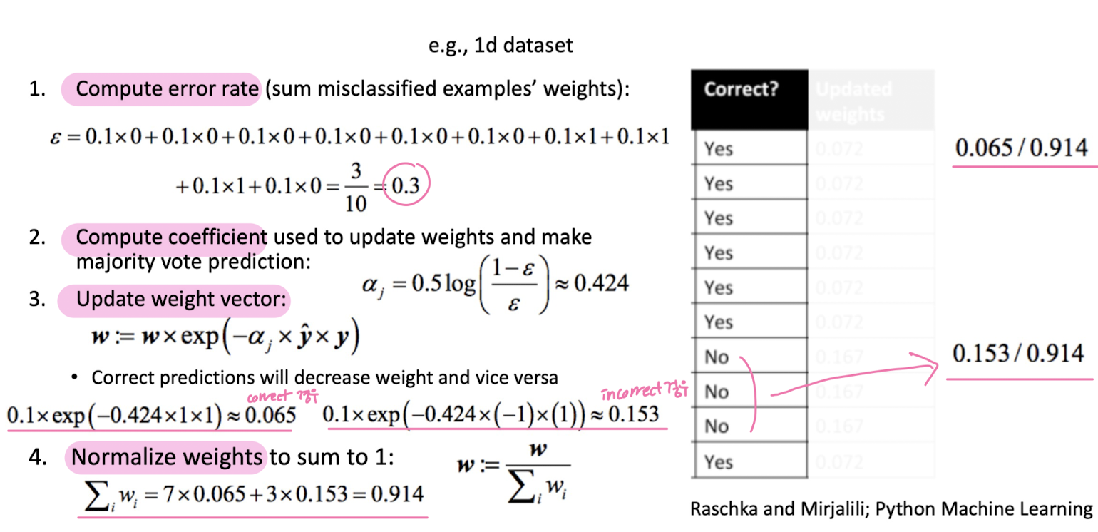
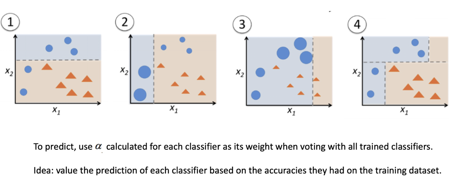
Boosting
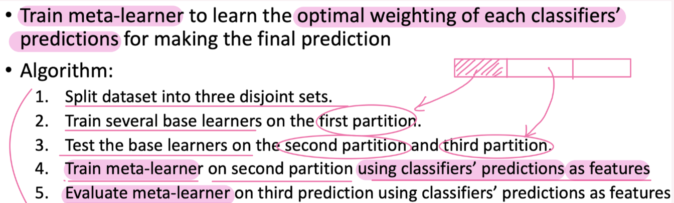
Stacking
- Stacking (Stackedm generaliztio) : Train a model that learns how to aggregate classifiers' predictions
7-2 ROC curve/ PR curve
-
Binary classification → Perceptron/ Adaline / Support Vector Machine
-
multiclass classification → Nearest Neighbor/ Decision Tree/ Naïve Bayes
-
Classifier confidence
-
Confusion Matrix for Binary Classification
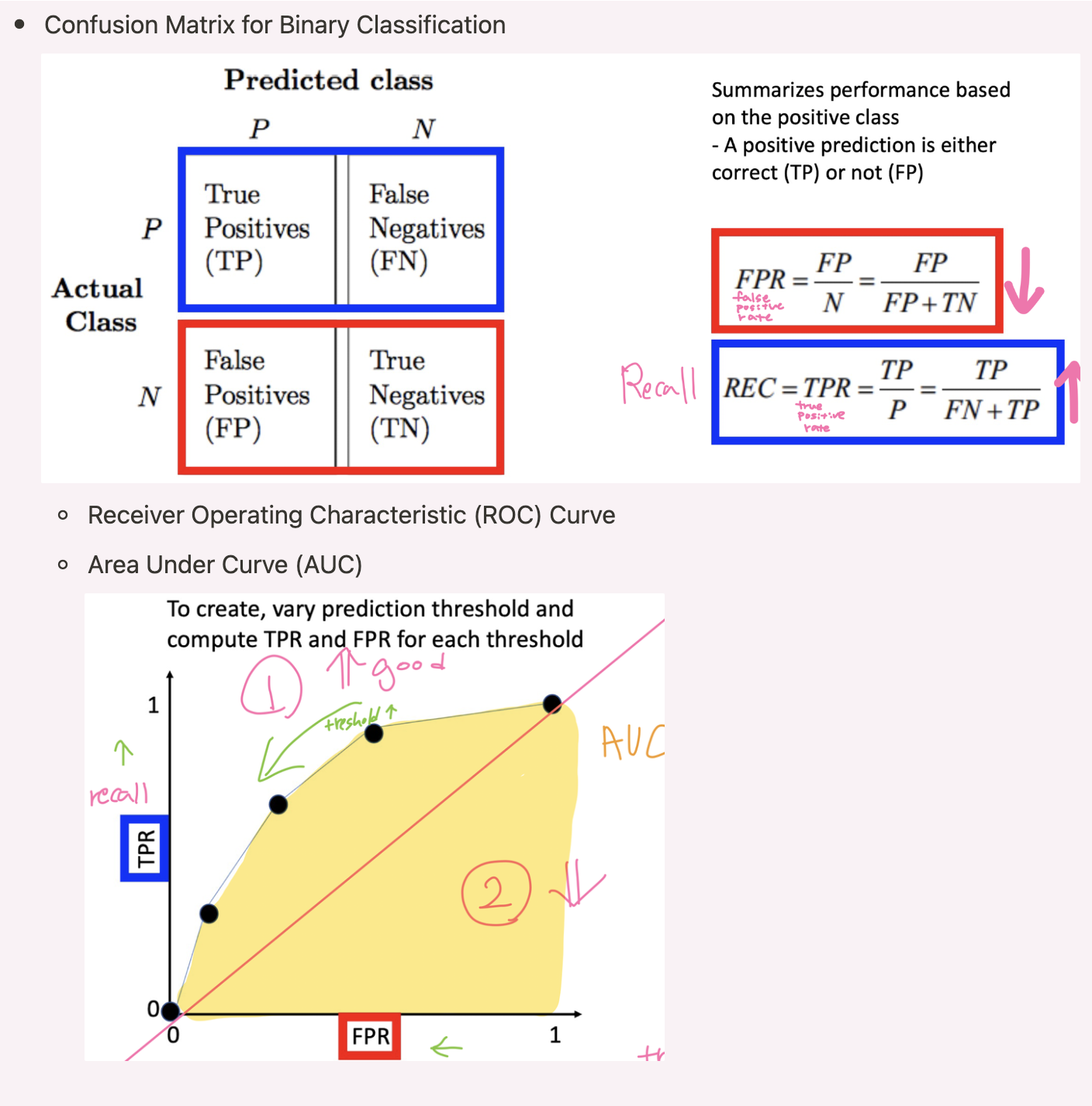
-
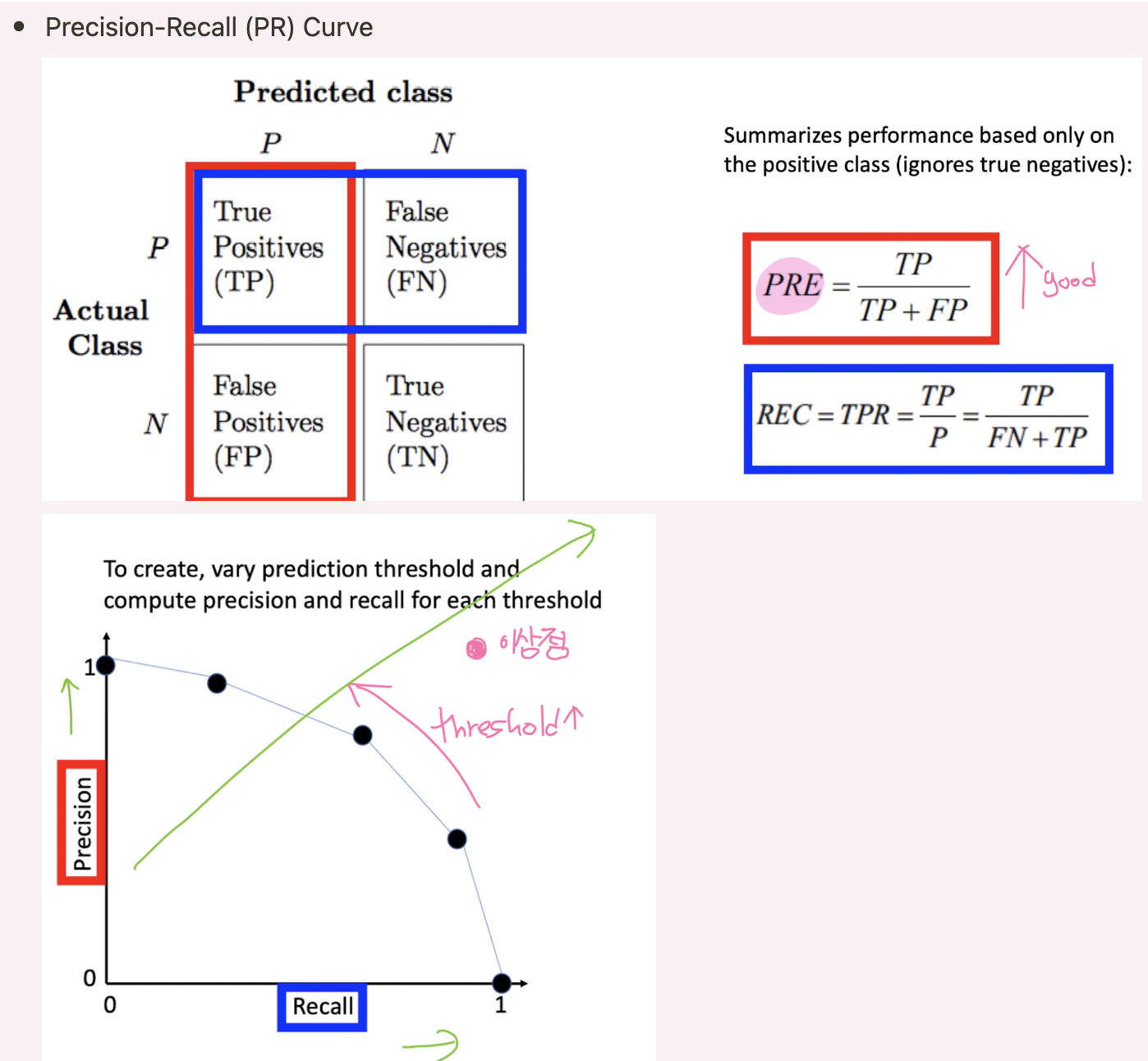
Precision-Recall (PR) Curve