[AI504] Class 04: Autoencoders

Latent representation

🔗 4-dimensional hidden representation

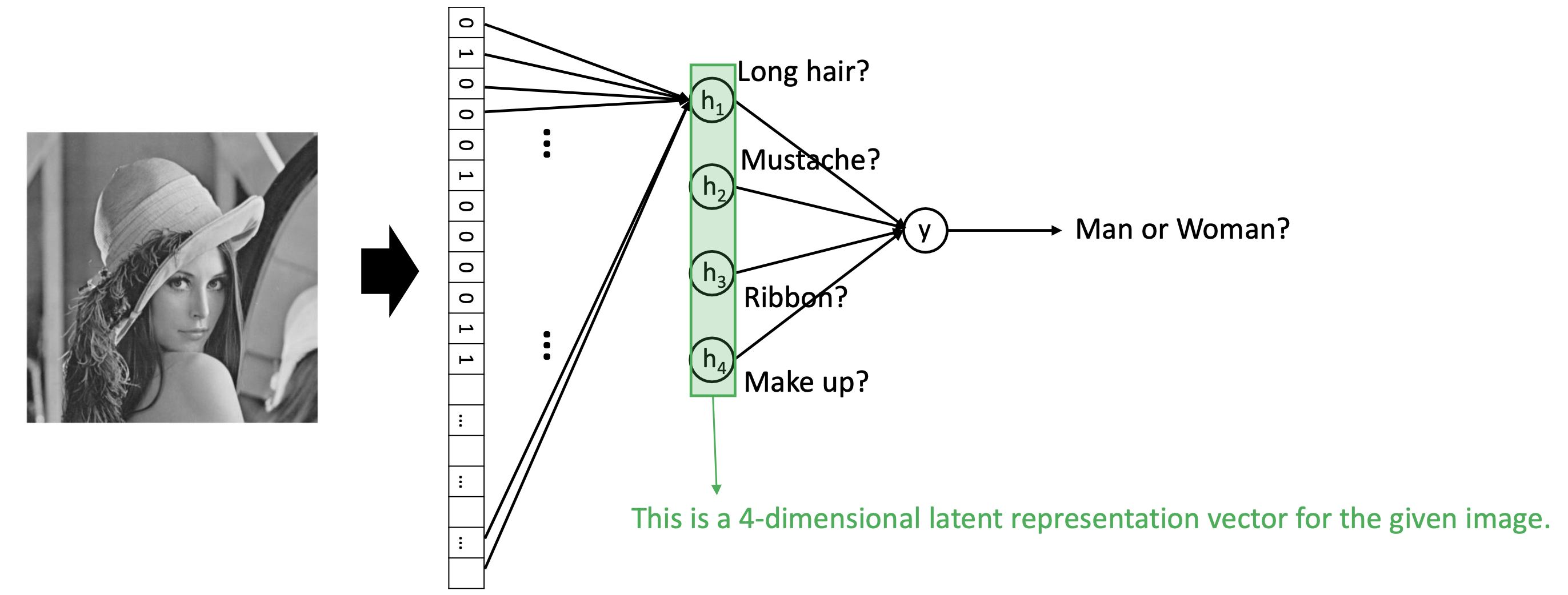
• latent representation = hidden representation = compressed representation
• 784 dimensional image가 4 dimensional space로 compress되었다.
• 4 dimensional space의 각 dimension은 final classification을 돕는 meaning을 가지고 있을 것이다. 사람에게는 해석이 안되는 걸수도, 되는 걸수도 있다.

🔗 Latent Representation

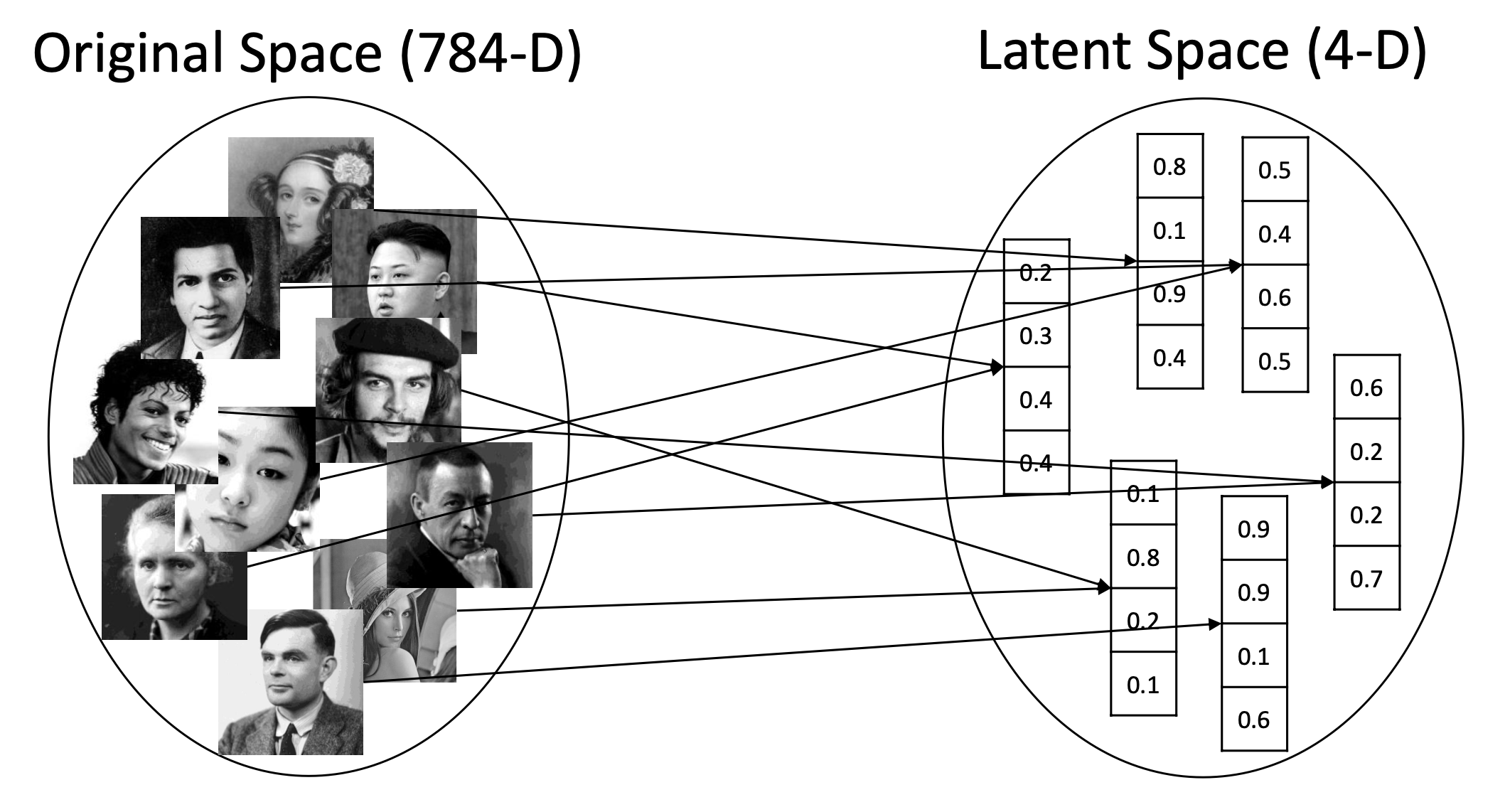
• 주어진 input sample을 compress하여 784d space에서 4d space로 mapping해주는 function이 있다.
• Original space와 latent space는 무한 집합(infinite set)이다.
• 이 function은 many-to-one relationship이 성립할 수 있다. 왜냐하면 dimension이 큰 쪽에서 작은 쪽으로 가기 때문에 아무래도 정보가 손실되고 압축되니까 동일한 것에 갈수도 있다. 하지만 실제로 완벽하게 같을 일은 없다.

🔗 Latent space를 어떻게 학습할까?

• Cross entropy loss를 minimize 시킴으로써 latent space를 학습한다.

❓ 왜 hidden layer를 써야하는가?

• Hidden layer는 non-linear task를 수행할 수 있도록 돕는다.

linear classifier : logistic regression, support vector machine등이 있다.

❓ 왜 non-linear activation을 써야하는가?

• 공간이 회전하고 늘고 줄고 선형으로 왼쪽 or 오른쪽으로 움직이는 것은 다 선형변환이고, 선형 변환만 해서는 non-linearity distributed data를 classify할 수 없다. 공간이 이상하게 찌그러지고 왜곡되는 비선형 변환을 해야지 선형 분류가 가능해진다.
• Non-linear transformation을 가진 input sample에 linear line을 그린다.
• Warping은 non-linear activation function이 수행한다.

❓ 두 group이 뒤얽혀 있어 linear transformation이나 non-linear activation function으로 100 accuracy를 얻지 못하는 경우에는 어떻게 해야할까?

• Higher dimension space에 mapping한다.
• 즉, model이 underfitting되었을 때, model의 capacity or power를 늘리거나 feature를 늘리는 조치를 취하는 것과 같은 것으로 해석할 수 있다.

🔗 Latent space

• Latent space는 loss function에 의해 결정된다/형성된다.
• Latent space는 function이 final task를 수행하기 위해서 intermediate layer에서 학습한 것이다.

오늘은 image compression task를 수행하여 형성된 latent space에 대해 배운다.

참고 사이트 : Neural Networks, Manifolds, and Topology

Autoencoders

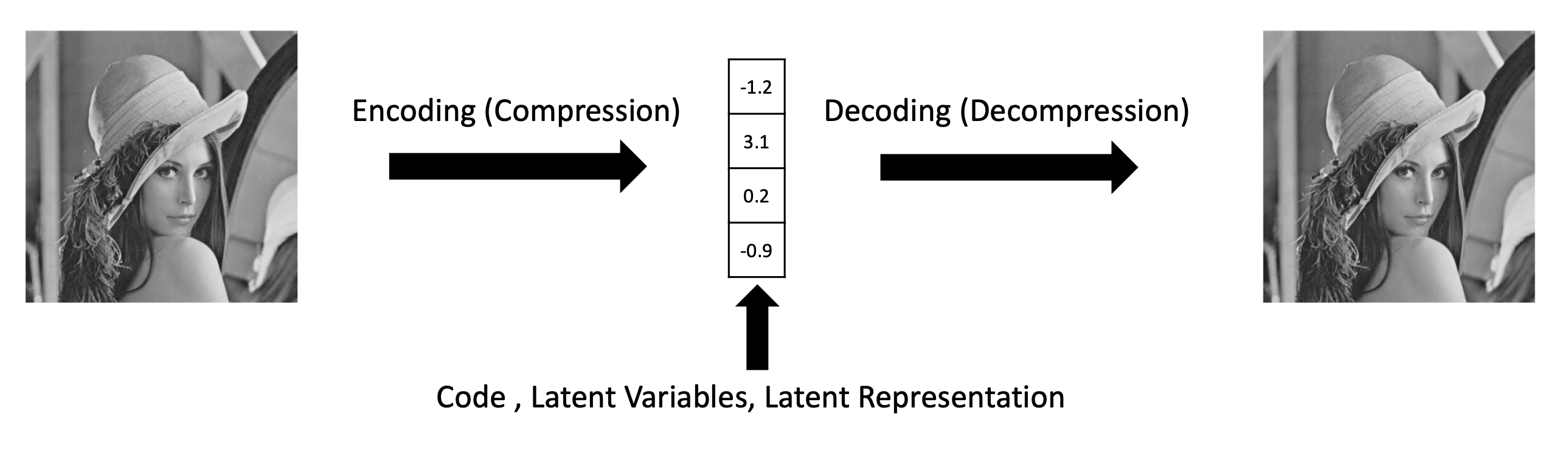
• Encoder와 decoder로 구성되어 있다.
• simple, symmetric architecture를 가지고 있다.

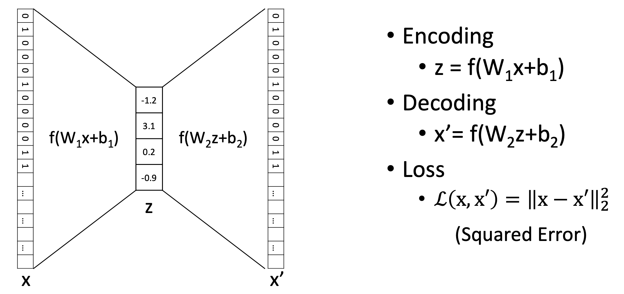
• Mean Squared Error (MSE) loss를 사용한다.- Mean Squared Error (MSE) loss를 사용한다.
• f는 non-linear activation function이다.
• f($W_1$x+$b_1$)과 f($W_2$x+$b_2$)는 single neural network hidden layer이다.
• $W_1$는 4*784 shape의, $W_2$는 784*4 shape의 matrix이어야한다.
• Autoencoder는 unsupervised learning이다(not supervised learning).
  • y label이 없으며, sample x가 label이 된다.
• 1개보다 더 많은 hidden layer를 사용할 수 있다.
  • Autoencoder를 RNN, CNN, Transformer등으로 만들 수도 있다.
  • 이때, 일반적으로 encoder와 decoder 사이에 가장 compressed된 space를 latent representation이라고 부른다.

🔗 Compression

• 784d에서 4d로 압축하는 것이기 때문에 information bottleneck이 존재한다.
• 따라서 약간의 uninformative, meaningless한 정보의 손실을 감안하더라도 useful하고 sample들 간에 가장 distinguish한 hidden feature만 4d space에 저장된다.
• Ex. background는 sample마다 차이가 거의 없는 meaningless한 information이라고 볼 수 있다. 따라서 background에 대한 정보는 compress할 때 기억할 필요 없는 정보이므로 소중한 4d space에 저장할 필요 없다.

❓ Autoencoder에 의해 형성된 4-dimension latent representation은 여전히 interpretable한 meaning을 가질까요?

• NO! Non-linear neural network로 학습했기 때문에 non-linearity가 적용되어 각 dimension에서 어떤 signal을 pick했는지 추측하기 매우 어렵다.
• 심지어 linear transformation function인 PCA로 얻어낸 learned principal component도 뭔지 해석하지 어렵다. 말할 것도 없이 autoencoder같은 non-linear transformation function에서의 learned component는 아마 해석할 수 없을 것이다.

🔗 Autoencoders VS PCA

✔️ 공통점

• Minimize reconstruction error == Maximize variance across different samples
• low variance(meaningless, not so distinguishing feature)는 버리고 오직 high variance(distinguishing) feature만 저장한다.

✔️ 차이점

• PCA
  • Linear transformation
  • PCA를 한 뒤에 내가 k개의 var-maximizing bases를 선택한다.
  • Higher dim space에 mapping하려면 kernal PCA를 사용해야한다.
• Autoencoder
  • Non-Linear transformation
  • train하기 전에 k dims(latent space size)를 미리 정의한다/결정한다.
  • Higher dim space에 mapping하려면 z=1000으로 설정함으로써 쉽게 할 수 있다.

🔗 Encoding to a higher dimensional space를 하면(dim(z)>dim(x)) MSE loss는 어떻게 될까?

• one-to-one corresponding을 할 수 있어 어떠한 compression도 일어나지 않고 information loss도 일어나지 않아 perfect reconstruction을 할 것이다.
• 양 쪽에서 identity function을 학습한다면, zero information zero loss로 reconstruct할 수 있다.

Training Process

항상 이 여섯 단계로 이루어져 있다.

① Split into train/validation/test
② Load data
③ Define a model M

• Define loss L

④ Define optimizer O
⑤ Training Loop
⑥ Evaluate best M on test set

Visualization

• Original space에서 비슷한 sample은 latent space에서도 여전히 비슷하다.
• 2d에 latent representation을 visualize하려면 추가적인 dimension reduction이 필요하다.
  • From dim(z) to 2

🔗 Popular algorithms for visualizing purposes

• PCA
  • linear transformation
  • variance-based compression
• t-SNE
  • sample간에 Local distance를 보존하려고 한다.
• UMAP
  • local distance뿐만 아니라 global structure도 조금 신경써서 보존하려고 한다.

보통 UMAP > t-SNE > PCA 이다.

참고 사이트 : Understanding UMAP

Autoencoder variants

2가지 유명한 variants가 있다.
🔗 Denoising autoencoder

• Induce sparse latent representations

• downstream classification에서 vanilla Autoencoder보다 성능이 좋다.

  • neural network에서 dropout과 같은 역할을 하여 sparsity를 야기한다. L1 regularization과 비슷하다.

• Latent space에 sparsity를 induce하고 싶으면 이 2가지 중 하나를 쓴다.

  1. KL-divergence
     

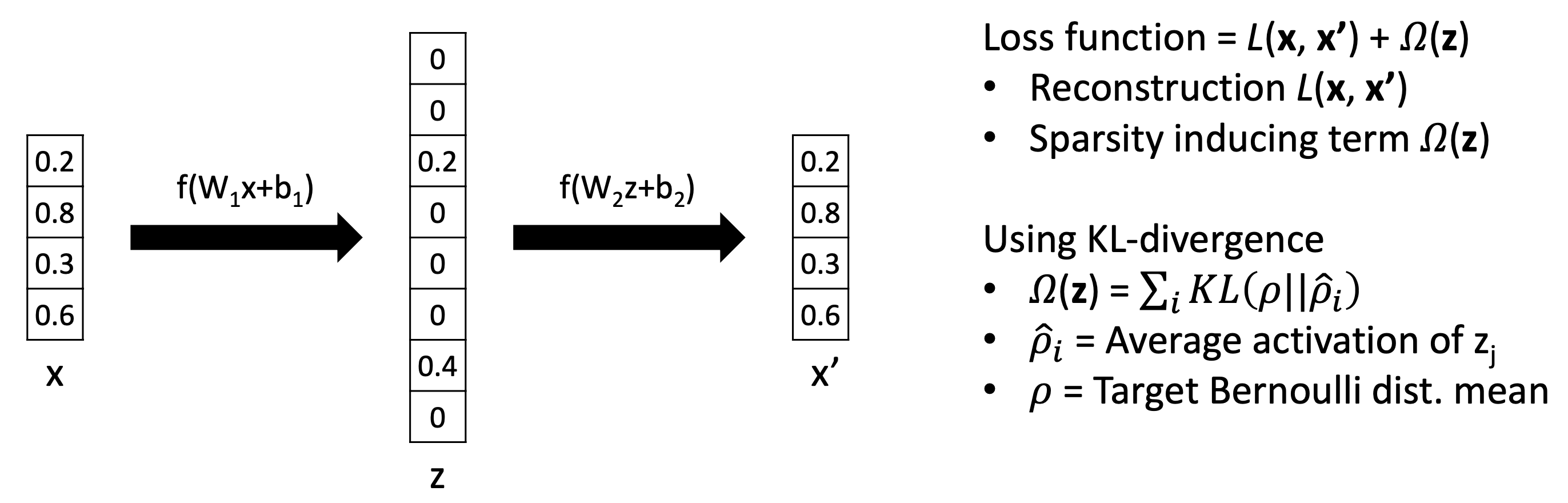
     • ρ : desire Bernoulli distribution
       • Ex. 0.1로 설정하면 해당하는 dimension은 10번 중 1번 activate하길 바란다.
     • ρ hat : individul dimension에 대해 얼마나 자주 activated되는지에 대한 empirical Bernoulli distribution

     Adjusting/controlling activity of each dimensionality

  2. L1 Regularization
     

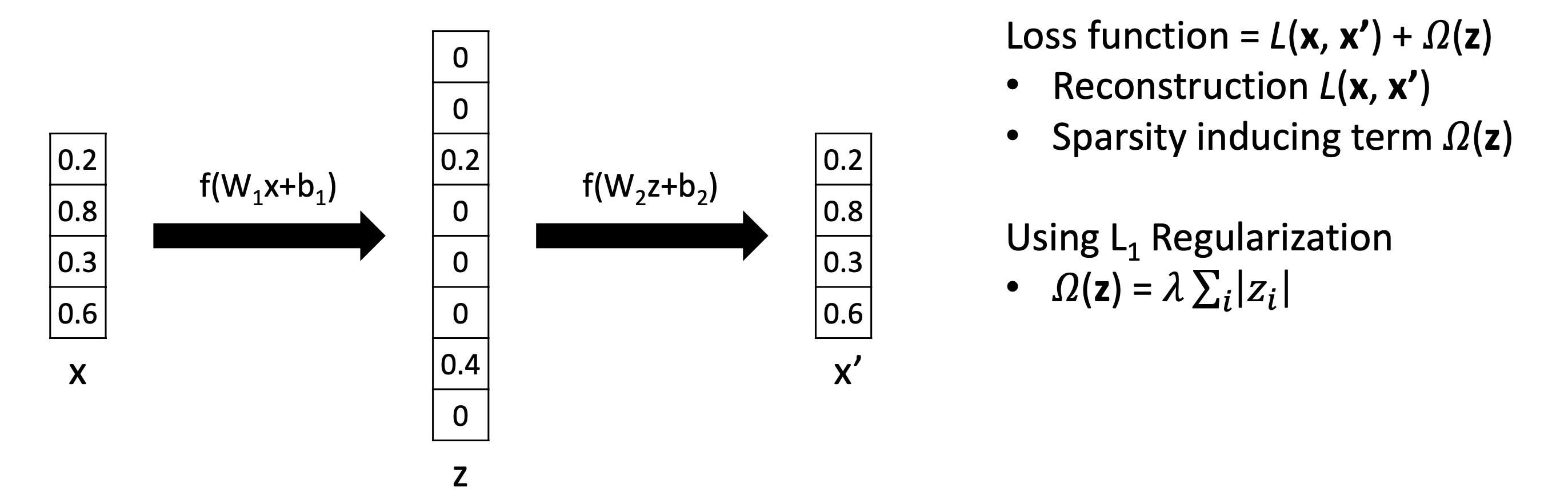
     L1 Regularization과 L2 Regularization의 차이
     0으로 갈때 L2는 error signal(loss)가 guadratically하게 감수해서 특정 point가 지나면 더이상 parameter를 update하지 않는다. 0으로 갈때 L1은 0이 될때까지 gradient가 1로 일정하다. 그래서 특정 point가 지나면 L1이 L2보다 더 peneralize한다. 그것이 L1이 sparsity를 induce하는 이유이다.

🔗 Sparse autoencoder

• Reconstruct an input with random noise

• 철학 : small noise는 higher-level representation에 영향을 주지 않는다.

  • Noise를 추가하면 noise는 information bottleneck에 의해 무시할만 하므로 별로 중요하지 않다. Noise는 small variance를 가지므로 무시된다.(Remind PCA!)

• Uncorrupted sample과 reconstruction sample 사이의 loss를 계산하기 때문에 latent space z는 corrupted sample을 denoise할 수 있을 만한 매우 robust한 latent representation을 학습한다. 그래서 latent space z는 test distribution에서 small variance/noise에 매우 robust하다.

• Downstream task를 하기에 useful하다.

  • Ex. classification, regression based on learned representation
  • End-to-end training이 아니고 denoising Autoencoder를 layer별로 train한다. 그리고서 얻은 final representation에 대해 예를 들어 10-way classifier를 한다.

Reference

• AI504: Programming for AI Lecture at KAIST AI