Autoencoder

1. Settings

1) Import required libraries

import numpy as np
import torch
import torch.nn as nn
import torch.optim as optim
import torch.nn.init as init
import torchvision.datasets as dset
import torchvision.transforms as transforms
from torch.utils.data import DataLoader
import matplotlib.pyplot as plt
import matplotlib as mpl

2) Set hyperparameters

batch_size = 256
learning_rate = 0.0002
num_epochs = 10

2. Data

1) Download Data

mnist_train = dset.MNIST("./", train=True, transform=transforms.ToTensor(), target_transform=None, download=True)
mnist_test = dset.MNIST("./", train=False, transform=transforms.ToTensor(), target_transform=None, download=True)
mnist_train, mnist_val = torch.utils.data.random_split(mnist_train, [50000, 10000])

mnist_train[0][0].size()    # (1, 28, 28) # (channel, height, width)

torch.Size([1, 28, 28])

mnist_train[0][1]           # label

6

2) Set DataLoader

dataloaders = {}
dataloaders['train'] = DataLoader(mnist_train, batch_size=batch_size, shuffle=True)
dataloaders['val'] = DataLoader(mnist_val, batch_size=batch_size, shuffle=False)
dataloaders['test'] = DataLoader(mnist_test, batch_size=batch_size, shuffle=False)

dataloaders.keys()

dict_keys(['train', 'val', 'test'])

len(dataloaders["train"])

196

3. Model & Optimizer

1) Model

# build your own autoencoder
# in my case: 784(1*28*28) -> 100 -> 30 -> 100 -> 784(28*28)

class Autoencoder(nn.Module):
    def __init__(self):
        super(Autoencoder,self).__init__()
        self.encoder = nn.Sequential(
            nn.Linear(28*28, 100),              # 여기에 CNN 등 다른 layer를 써도 된다.
            nn.ReLU(),                          # activation function
            nn.Linear(100, 30),
            nn.ReLU()                           # activation function
        )
        
        self.decoder = nn.Sequential(
            nn.Linear(30, 100),
            nn.ReLU(),                          # activation function
            nn.Linear(100, 28*28),
            nn.Sigmoid()                          # activation function
        )

                
    def forward(self, x):                # x: (batch_size, 1, 28, 28)
        batch_size = x.size(0)
        x = x.view(-1, 28*28)                          # reshape to 784(28*28)-dimensional vector
        encoded = self.encoder(x)                    # hidden vector
        out = self.decoder(encoded).view(batch_size, 1, 28, 28)                        # final output. resize to input's size
        return out, encoded

Linear layer는 오직 마지막 element(784)에만 적용된다. 그래서 Autoencoder의 앞 단계에서는 batch size를 고려하지 않아도 된다.

model을 train하거나 validate할 때 batch-wise operation을 한다.
x = (B, C, W, H)
x.view(-1, W*H) => x.shape == (B*C, W*H)
x.view(B, -1, W, H) => x.shape == (B, C, W, H)

MNIST dataset에 있는 tensor의 모든 element가 0과 1사이에 있기 때문에 output space를 (0,1)로 제한하기 위해서 마지막에 sigmoid non-linearity function을 쓴다.

(mnist_train[1][0] <= 1).sum()

tensor(784)

Reshape function과 view function의 차이점
locating memory issue이다. 두 function은 비슷하게 동작하지만, function이 contiguous = True tensors로 적용될 수 있는가의 여부에 차이점이 있다.

Contiguous
Tensor의 각 element가 컴퓨터 메모리에 할당될때 메모리 주소가 이전 주소의 바로 다음이라는 것이다.
1,2,3,4 : contiguous
1,(2),3,(4),5,(6),7 : not-contiguous

2) Loss func & Optimizer

device = torch.device("cuda:0" if torch.cuda.is_available() else "cpu")
print(device)

cuda:0

model = Autoencoder().to(device)
loss_func = nn.MSELoss()
optimizer = torch.optim.Adam(model.parameters(), lr=learning_rate)

4. Train

import time
import copy

def train_model(model, dataloaders, criterion, optimizer, num_epochs=10):
    """
    model: model to train
    dataloaders: train, val, test data's loader
    criterion: loss function
    optimizer: optimizer to update your model
    """
    since = time.time()

    train_loss_history = []
    val_loss_history = []

    best_model_wts = copy.deepcopy(model.state_dict())
    best_val_loss = 100000000

    for epoch in range(num_epochs):
        print('Epoch {}/{}'.format(epoch, num_epochs - 1))
        print('-' * 10)

        # Each epoch has a training and validation phase
        for phase in ['train', 'val']:
            if phase == 'train':
                model.train()            # Set model to training mode
            else:
                model.eval()            # Set model to evaluate mode

            running_loss = 0.0

            # Iterate over data.
            for inputs, labels in dataloaders[phase]:
                inputs = inputs.to(device)                                       # transfer inputs to GPU 

                # zero the parameter gradients
                optimizer.zero_grad()

                # forward
                # track history if only in train
                with torch.set_grad_enabled(phase == 'train'):

                    outputs, encoded = model(inputs)
                    loss = criterion(outputs, inputs)                          # calculate a loss


                    # backward + optimize only if in training phase
                    if phase == 'train':
                        loss.backward()                             # perform back-propagation from the loss
                        optimizer.step()                             # perform gradient descent with given optimizer

                # statistics
                running_loss += loss.item() * inputs.size(0)                    

            epoch_loss = running_loss / len(dataloaders[phase].dataset)

            print('{} Loss: {:.4f}'.format(phase, epoch_loss))
            
            # deep copy the model
            if phase == 'train':
                train_loss_history.append(epoch_loss)
            
            if phase == 'val':
                val_loss_history.append(epoch_loss)

            if phase == 'val' and epoch_loss < best_val_loss:
                best_val_loss = epoch_loss
                best_model_wts = copy.deepcopy(model.state_dict())
                
            
        print()

    time_elapsed = time.time() - since
    print('Training complete in {:.0f}m {:.0f}s'.format(time_elapsed // 60, time_elapsed % 60))
    print('Best val Loss: {:4f}'.format(best_val_loss))

    # load best model weights
    model.load_state_dict(best_model_wts)
    return model, train_loss_history, val_loss_history

best_model, train_loss_history, val_loss_history = train_model(model, dataloaders, loss_func, optimizer, num_epochs=num_epochs)

Epoch 0/9
----------
train Loss: 0.1174
val Loss: 0.0700

Epoch 1/9
----------
train Loss: 0.0647
val Loss: 0.0588

Epoch 2/9
----------
train Loss: 0.0541
val Loss: 0.0481

Epoch 3/9
----------
train Loss: 0.0435
val Loss: 0.0404

Epoch 4/9
----------
train Loss: 0.0391
val Loss: 0.0369

Epoch 5/9
----------
train Loss: 0.0353
val Loss: 0.0333

Epoch 6/9
----------
train Loss: 0.0319
val Loss: 0.0302

Epoch 7/9
----------
train Loss: 0.0293
val Loss: 0.0280

Epoch 8/9
----------
train Loss: 0.0274
val Loss: 0.0264

Epoch 9/9
----------
train Loss: 0.0258
val Loss: 0.0248

Training complete in 1m 15s
Best val Loss: 0.024841

# Let's draw a learning curve like below.
plt.plot(train_loss_history, label='train')
plt.plot(val_loss_history, label='val')
plt.xlabel('epoch')
plt.ylabel('loss')
plt.legend()
plt.show()
# overfitting이 보이지 않는다.
# 9 epoch으로는 완전하게 훈련하기 충분하지 않다는 것을 알 수 있다.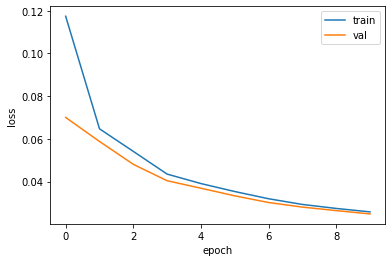

5. Check with Test Image

with torch.no_grad():
    running_loss = 0.0
    for inputs, labels in dataloaders["test"]:
        inputs = inputs.to(device)

        outputs, encoded = best_model(inputs)
        test_loss = loss_func(outputs, inputs)
        
        running_loss += test_loss.item() * inputs.size(0)

    test_loss = running_loss / len(dataloaders["test"].dataset)
    print(test_loss)        

0.02449837400317192

out_img = torch.squeeze(outputs.cpu().data)
print(out_img.size())

for i in range(5):
    plt.subplot(1,2,1)
    plt.imshow(torch.squeeze(inputs[i]).cpu().numpy(),cmap='gray')
    plt.subplot(1,2,2)
    plt.imshow(out_img[i].numpy(),cmap='gray')
    plt.show()

torch.Size([16, 28, 28])

6. Visualizing MNIST

np.random.seed(42)

from sklearn.manifold import TSNE

test_dataset_array = mnist_test.data.numpy() / 255
test_dataset_array = np.float32(test_dataset_array)
labels = mnist_test.targets.numpy()

test_dataset_array = torch.tensor(test_dataset_array)
inputs = test_dataset_array.to(device)
outputs, encoded = best_model(inputs)

encoded = encoded.cpu().detach().numpy()
tsne = TSNE()   
X_test_2D = tsne.fit_transform(encoded)
X_test_2D = (X_test_2D - X_test_2D.min()) / (X_test_2D.max() - X_test_2D.min())

plt.scatter(X_test_2D[:, 0], X_test_2D[:, 1], c=labels, s=10, cmap="tab10")
plt.axis("off")
plt.show()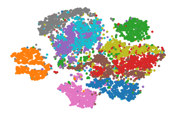

Let's make this diagram a bit prettier:

# adapted from https://scikit-learn.org/stable/auto_examples/manifold/plot_lle_digits.html
plt.figure(figsize=(10, 8))
cmap = plt.cm.tab10
plt.scatter(X_test_2D[:, 0], X_test_2D[:, 1], c=labels, s=10, cmap=cmap)
image_positions = np.array([[1., 1.]])
for index, position in enumerate(X_test_2D):
    dist = np.sum((position - image_positions) ** 2, axis=1)
    if np.min(dist) > 0.02: # if far enough from other images
        image_positions = np.r_[image_positions, [position]]
        imagebox = mpl.offsetbox.AnnotationBbox(
            mpl.offsetbox.OffsetImage(torch.squeeze(inputs).cpu().numpy()[index], cmap="binary"),
            position, bboxprops={"edgecolor": cmap(labels[index]), "lw": 2})
        plt.gca().add_artist(imagebox)
plt.axis("off")
plt.show()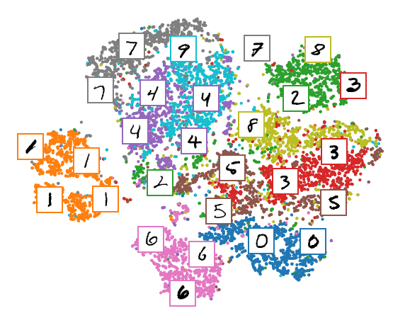

Denoising Autoencoder

model_D = Autoencoder().to(device)
loss_func = nn.MSELoss()
optimizer = torch.optim.Adam(model_D.parameters(), lr=learning_rate)

# It's all the same except for one: adding noise to inputs
# copy train_model() code and just add 'noise part'
# Hint: You can make noise like this.
# noise = torch.zeros(inputs.size(0), 1, 28, 28)
# nn.init.normal_(noise, 0, 0.1)

def train_model_D(model, dataloaders, criterion, optimizer, num_epochs=10):

  """
  model: model to train
  dataloaders: train, val, test data's loader
  criterion: loss function
  optimizer: optimizer to update your model
  """
  since = time.time()

  train_loss_history = []
  val_loss_history = []

  best_model_wts = copy.deepcopy(model.state_dict())
  best_val_loss = 100000000

  for epoch in range(num_epochs):
      print('Epoch {}/{}'.format(epoch, num_epochs - 1))
      print('-' * 10)

      # Each epoch has a training and validation phase
      for phase in ['train', 'val']:
          if phase == 'train':
              model.train()            # Set model to training mode
          else:
              model.eval()            # Set model to evaluate mode

          running_loss = 0.0

          # Iterate over data.
          for inputs, labels in dataloaders[phase]:
              inputs = inputs.to(device)
              noise = torch.zeros(inputs.size(0), 1, 28, 28)
              nn.init.normal_(noise, 0, 0.1)
              noise = noise.to(device)
              noise_inputs = inputs + noise                     # transfer inputs to GPU 

              # zero the parameter gradients
              optimizer.zero_grad()

              # forward
              # track history if only in train
              with torch.set_grad_enabled(phase == 'train'):

                  outputs, encoded = model(noise_inputs)
                  loss = criterion(outputs, inputs)                          # calculate a loss


                  # backward + optimize only if in training phase
                  if phase == 'train':
                      loss.backward()                             # perform back-propagation from the loss
                      optimizer.step()                             # perform gradient descent with given optimizer

              # statistics
              running_loss += loss.item() * inputs.size(0)                    

          epoch_loss = running_loss / len(dataloaders[phase].dataset)

          print('{} Loss: {:.4f}'.format(phase, epoch_loss))
            
          # deep copy the model
          if phase == 'train':
              train_loss_history.append(epoch_loss)
            
          if phase == 'val':
              val_loss_history.append(epoch_loss)

          if phase == 'val' and epoch_loss < best_val_loss:
              best_val_loss = epoch_loss
              best_model_wts = copy.deepcopy(model.state_dict())
                
            
      print()

  time_elapsed = time.time() - since
  print('Training complete in {:.0f}m {:.0f}s'.format(time_elapsed // 60, time_elapsed % 60))
  print('Best val Loss: {:4f}'.format(best_val_loss))

  # load best model weights
  model.load_state_dict(best_model_wts)
    
  return model, train_loss_history, val_loss_history

best_model_D, train_loss_history_D, val_loss_history_D = train_model_D(model_D, dataloaders, loss_func, optimizer, num_epochs=num_epochs)

Epoch 0/9
----------
train Loss: 0.1125
val Loss: 0.0696

Epoch 1/9
----------
train Loss: 0.0646
val Loss: 0.0593

Epoch 2/9
----------
train Loss: 0.0544
val Loss: 0.0482

Epoch 3/9
----------
train Loss: 0.0439
val Loss: 0.0405

Epoch 4/9
----------
train Loss: 0.0392
val Loss: 0.0373

Epoch 5/9
----------
train Loss: 0.0357
val Loss: 0.0335

Epoch 6/9
----------
train Loss: 0.0321
val Loss: 0.0304

Epoch 7/9
----------
train Loss: 0.0293
val Loss: 0.0280

Epoch 8/9
----------
train Loss: 0.0269
val Loss: 0.0257

Epoch 9/9
----------
train Loss: 0.0250
val Loss: 0.0240

Training complete in 1m 19s
Best val Loss: 0.024009

plt.plot(train_loss_history_D, label='train')
plt.plot(val_loss_history_D, label='val')
plt.xlabel('epoch')
plt.ylabel('loss')
plt.legend()
plt.show()
# 모델이 아직 충분히 train되지 않았다는 것을 의미한다.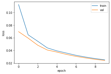

with torch.no_grad():
  running_loss = 0.0
  for inputs, labels in dataloaders['test']:
      noise = nn.init.normal_(torch.FloatTensor(inputs.size(0), 1, 28, 28), 0, 0.1)
      noise = noise.to(device)
      inputs = inputs.to(device)
      noise_inputs = inputs + noise

      outputs, encoded = best_model_D(noise_inputs)
      test_loss = loss_func(outputs, inputs)
      
      running_loss += test_loss.item()* inputs.size(0)

  test_loss = running_loss / len(dataloaders['test'].dataset)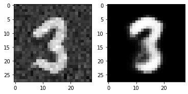
  print(test_loss) 

0.023626958617568018

out_img = torch.squeeze(outputs.cpu().data)
print(out_img.size())

for i in range(5):
    plt.subplot(1,2,1)
    plt.imshow(torch.squeeze(noise_inputs[i]).cpu().numpy(),cmap='gray')
    plt.subplot(1,2,2)
    plt.imshow(out_img[i].numpy(),cmap='gray')
    plt.show()

torch.Size([16, 28, 28])

Reference

• AI504: Programming for AI Lecture at KAIST AI