[AI504] Class 13: Deep Diffusion Probabilistic Model

Generative Model Recap

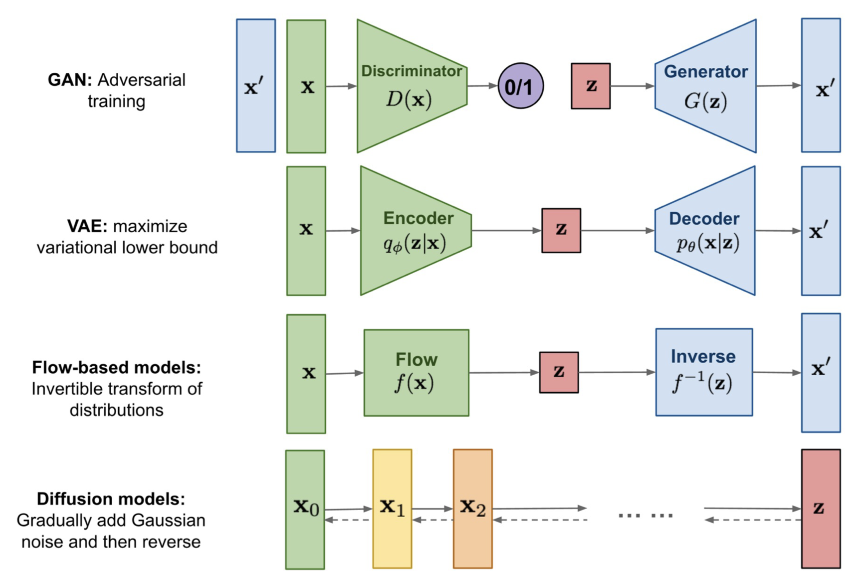
• Autoregressive Models
  • generate a sample in a sequential manner.

VAEs, Flow-based models, Autoregressive models 모두 이미 아는 distribution에서 sampling하여 이 sample을 original image/sample space로 mapping하고 싶은 것이다.

DDPM

Diffusion

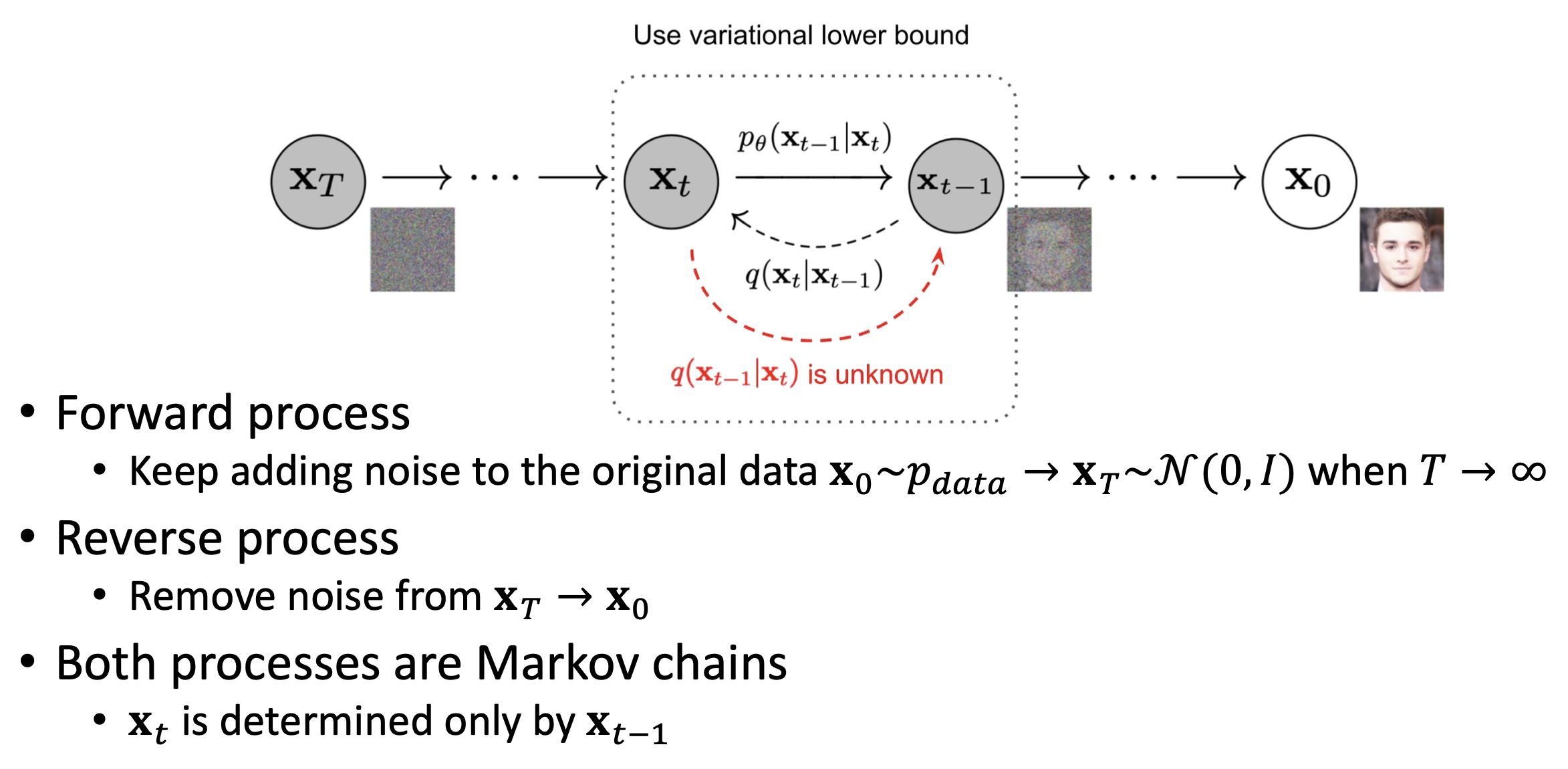
• Forward process와 backward process 모두 Markov assumption을 따른다.

Forward Process

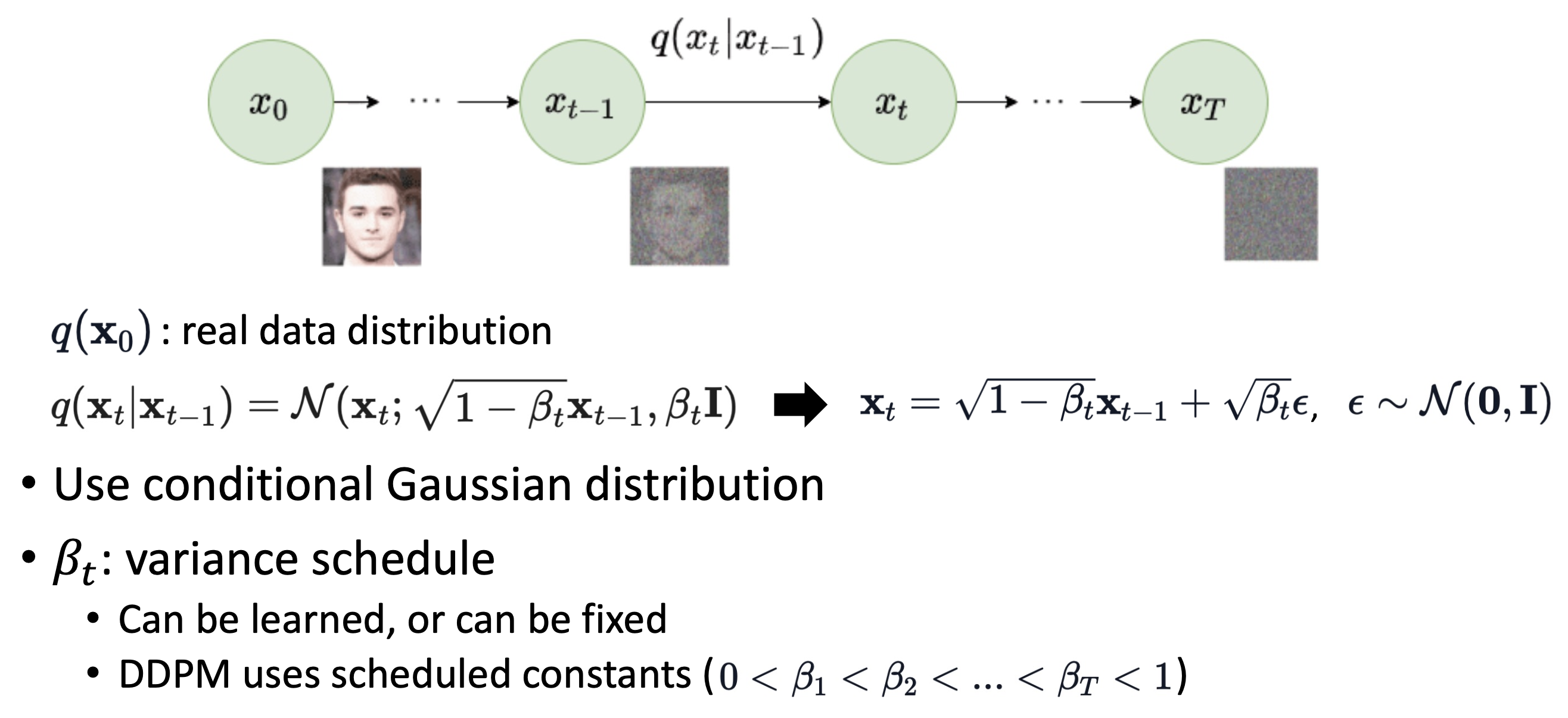
• β가 매우매우 작은 scaler value이면, $x_t$이 $x_{t-1}$과 크게 다르지 않다는 것을 의미한다. $x_{t-1}$에서 매우 작은 noise를 추가해서 $x_t$를 얻을 수 있다.

• 즉, 어떤 sample이든 작은 gaussian noise를 반복적으로 더함으로써 learnable parameter 없이 N(0,I)로 변환할 수 있다.

• Reparameterization trick
  x ~ N(μ, σ)
  x = μ + σ*ε
  ε ~ N(0, I)
  

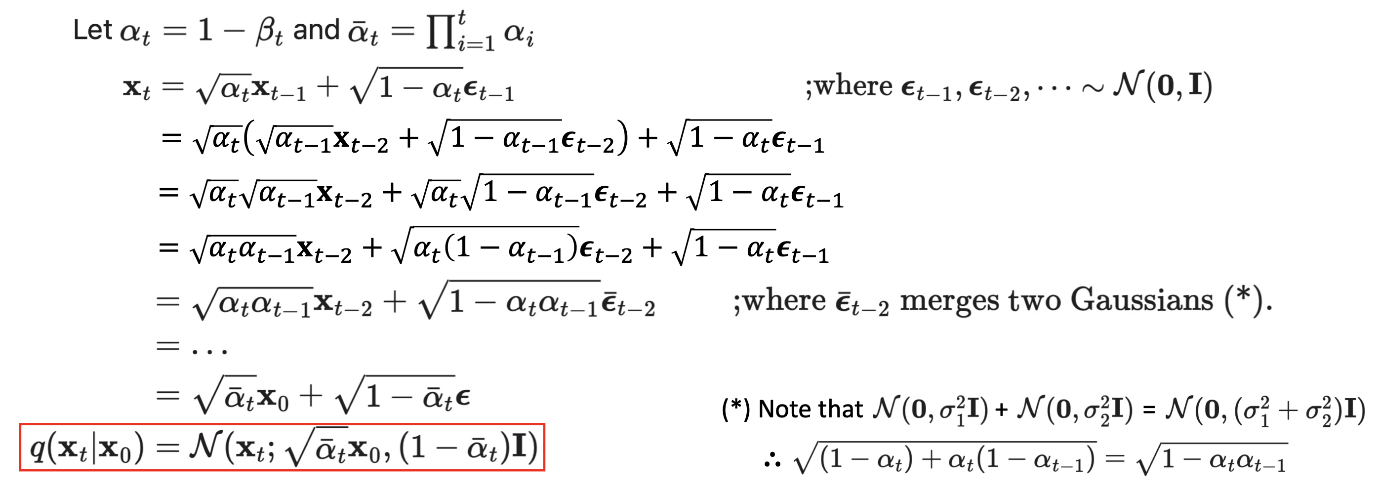
🔗 Creating $x_t$ straight from $x_0$

$x_t$를 구하기 위해 반복적으로 noise를 더하지 않아도 $x_0$로부터 바로 구할 수 있다.

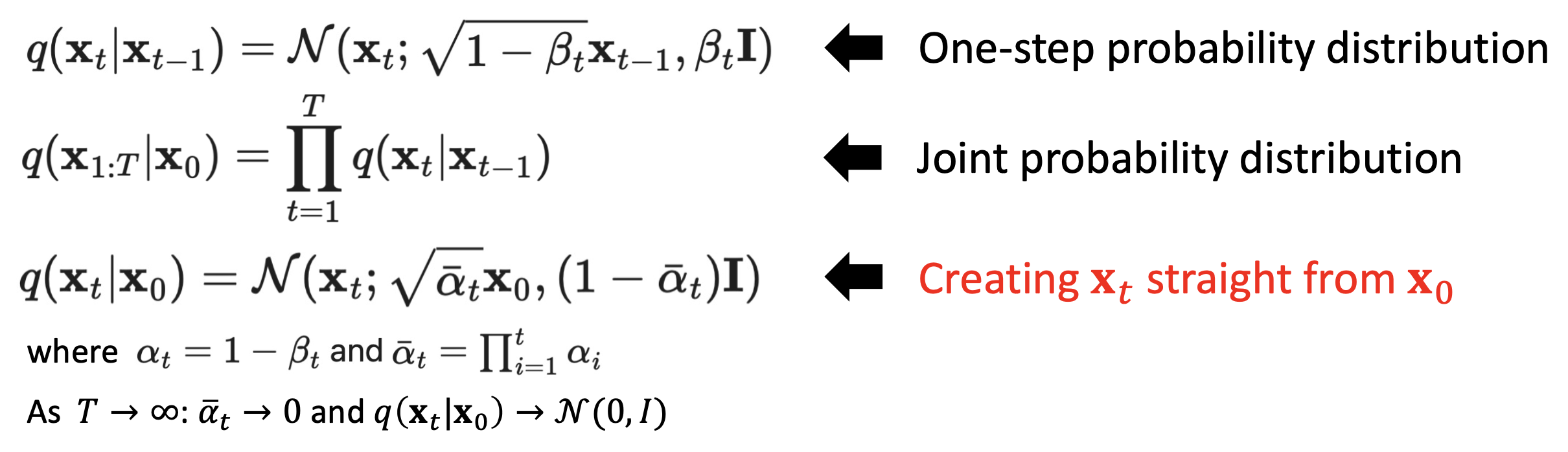
• Originally, DDPM predicts mean of gaussian but by using this nice property, we can reparameterize training objective to let the model predict epsilon. And it works better. This is why we called this property as a nice property.

✔️ 전개 과정

Reverse Process

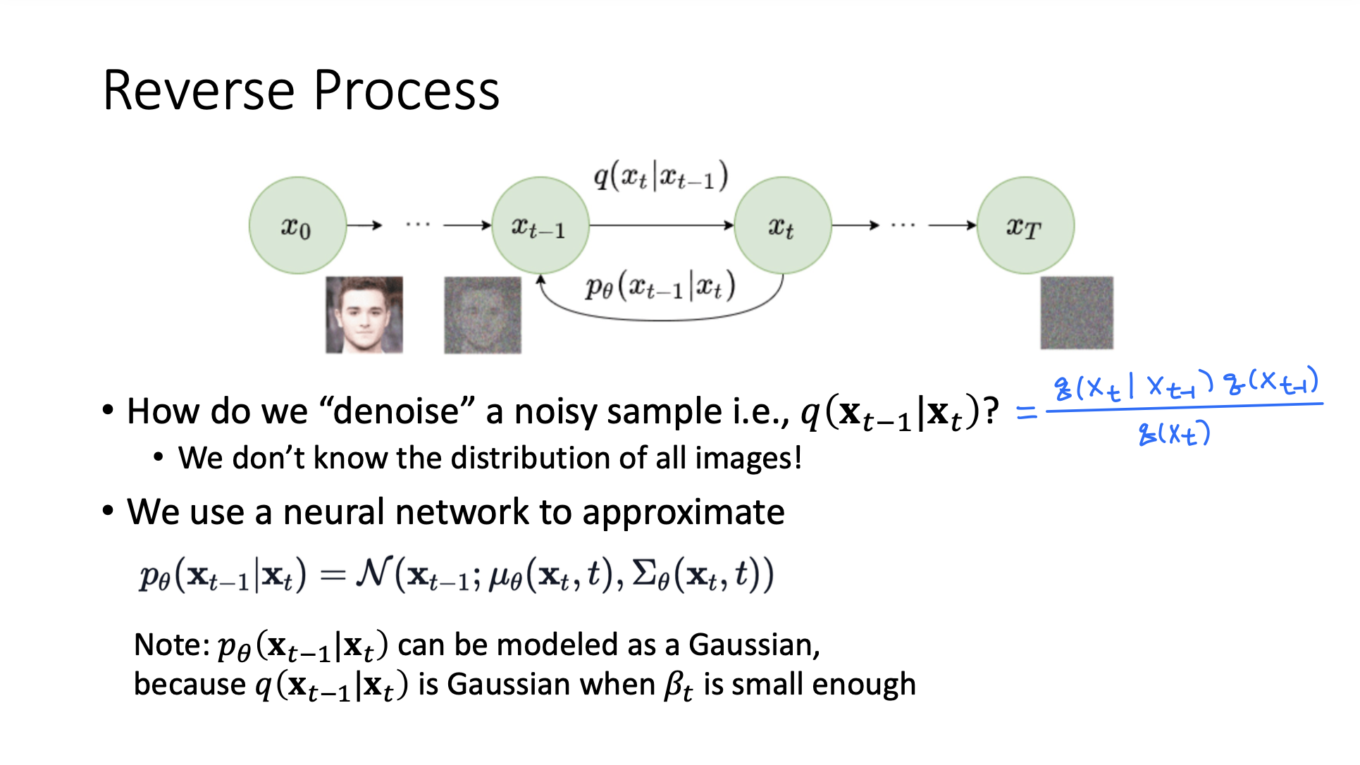
• q($x_{t-1}$), q($x_t$) : distribution over all images with some level of noise
  • Intractable! 계산할 수 없다.

➡️ 그래서 neural network를 사용해 approximate한다.

• 이론적으로, q($x_t$|$x_{t-1}$)가 Gaussian일 때, β가 매우 작으면 q($x_{t-1}$|$x_t$)도 Gaussian이다.

➡️ Gaussian으로 approximate한다. 그러므로 이제 neural network를 통해 μ와 σ를 estimate해야한다.

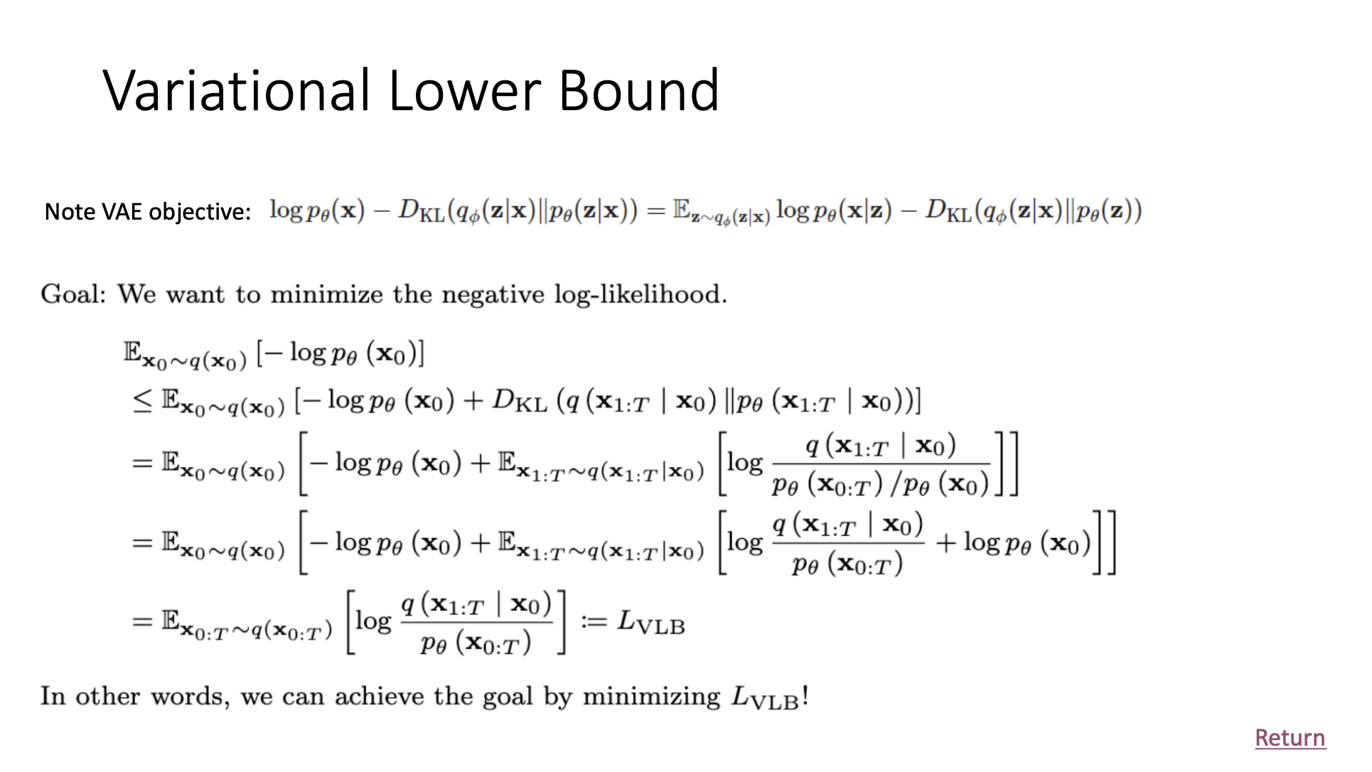
🔗 How do we train $p_θ$($x_{t-1}$|$x_t$)?

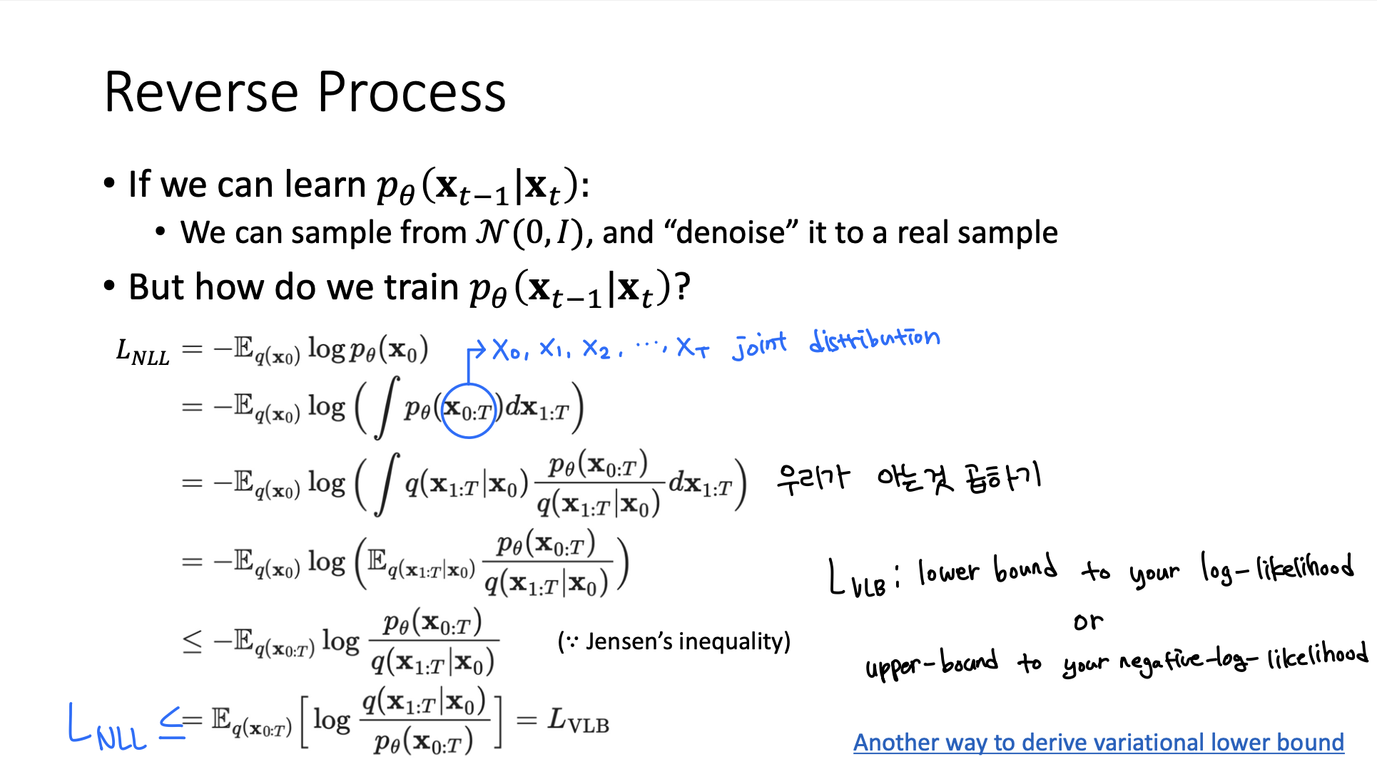
➡️ Variational Lower Bound $L_{VLB}$를 optimize함으로써, $p_θ$($x_{t-1}$|$x_t$)를 학습할 수 있다. 나머지 부분은 모두 우리가 아는 gaussian distribution이다.

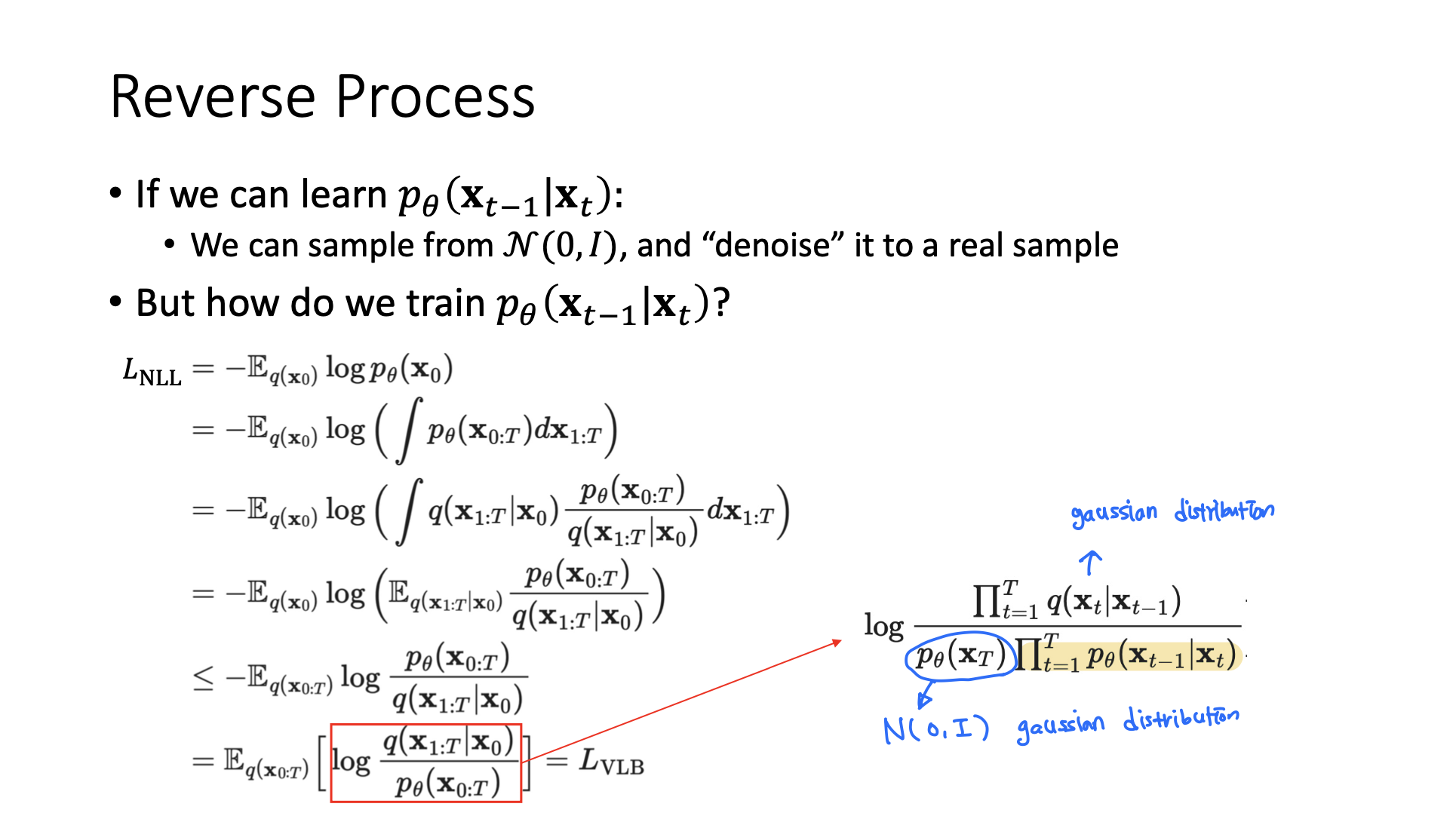
하지만 이 formula로 간다면, $x_0$을 뽑아서 $x_0$, $x_0$, ..., $x_0$까지 모두 계산한 다음 optimize해야한다. 이렇게 되면 variance가 높아질 수 있다. 그래서 $L_{VLB}$를 세 부분으로 더 나눈다.
이렇게 하여 $p_θ$ model을 training하는 동안 variance를 낮출 수 있다.

🔗 Further break down of $L_{VLB}$ to reduce variance

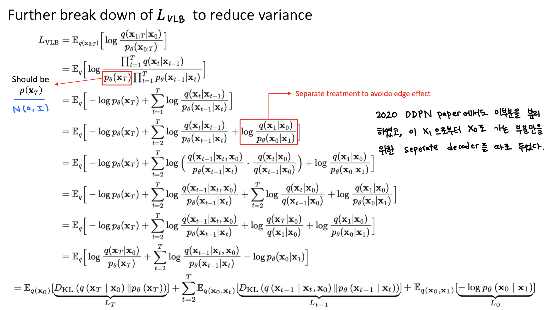
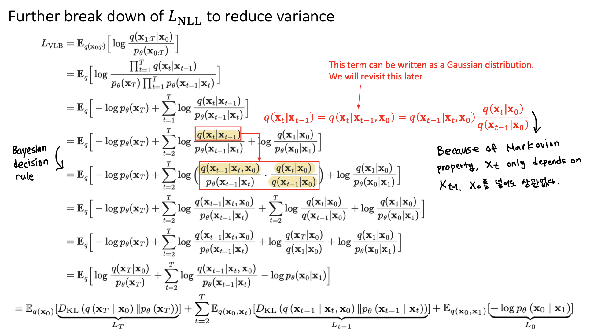
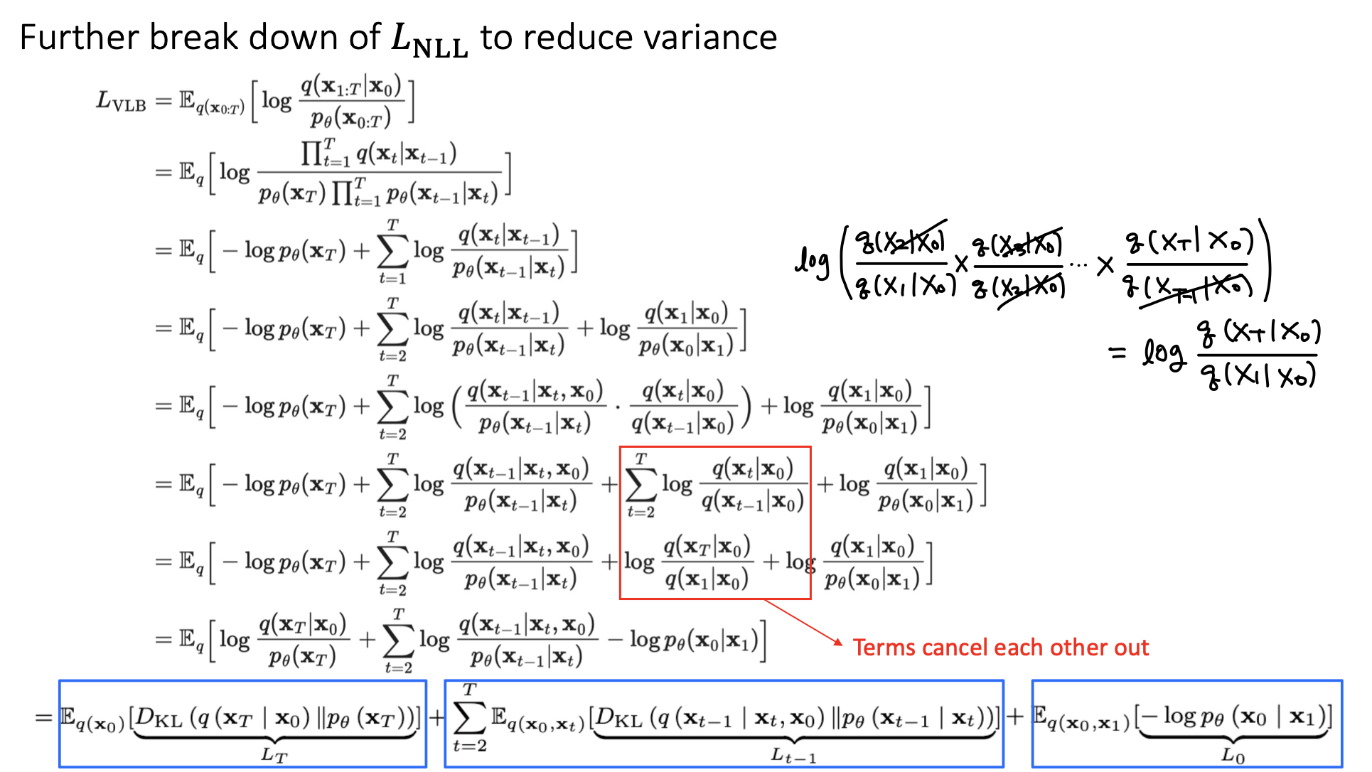
• 두 gaussian distribution 사이의 KL Divergence는 analytically tractable! 모두 다 두 gaussian distribution 사이의 KL Divergence이다.

🔗 Looking at Each Term

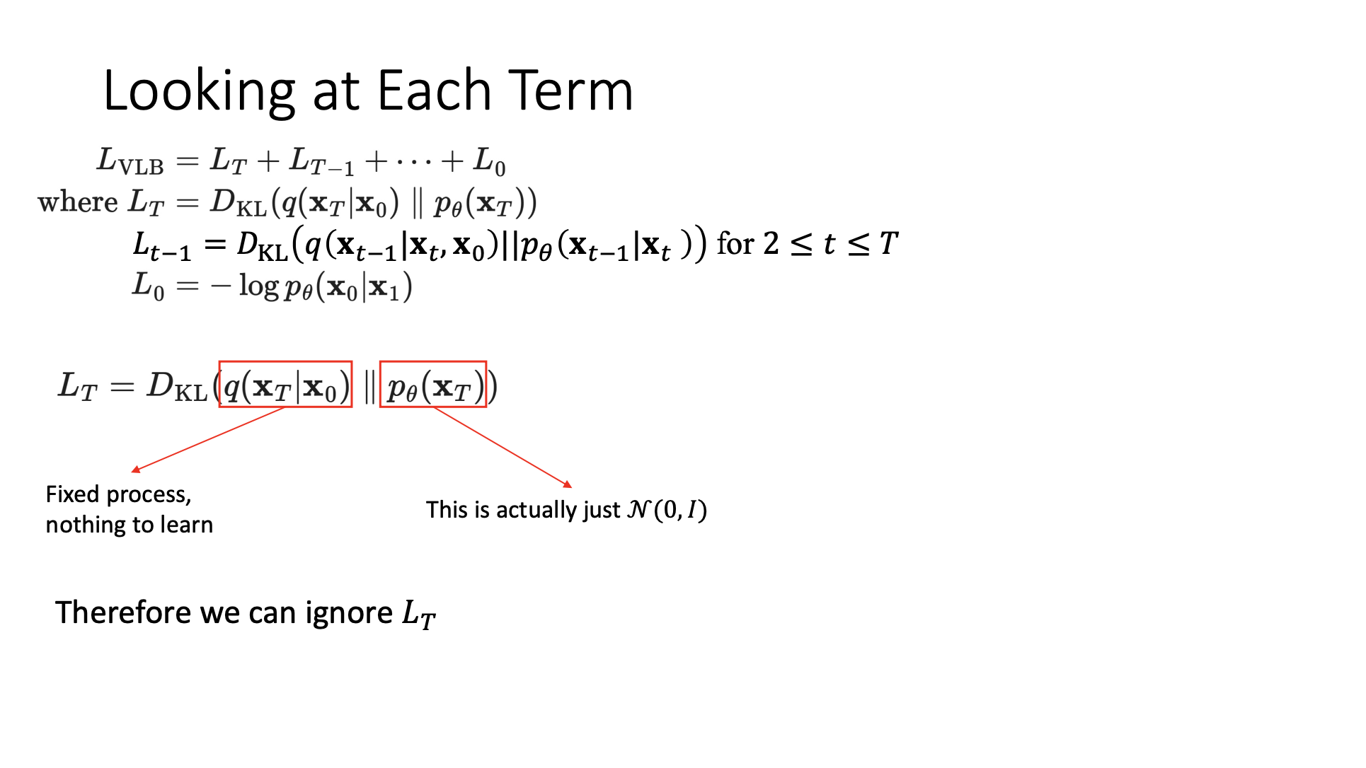
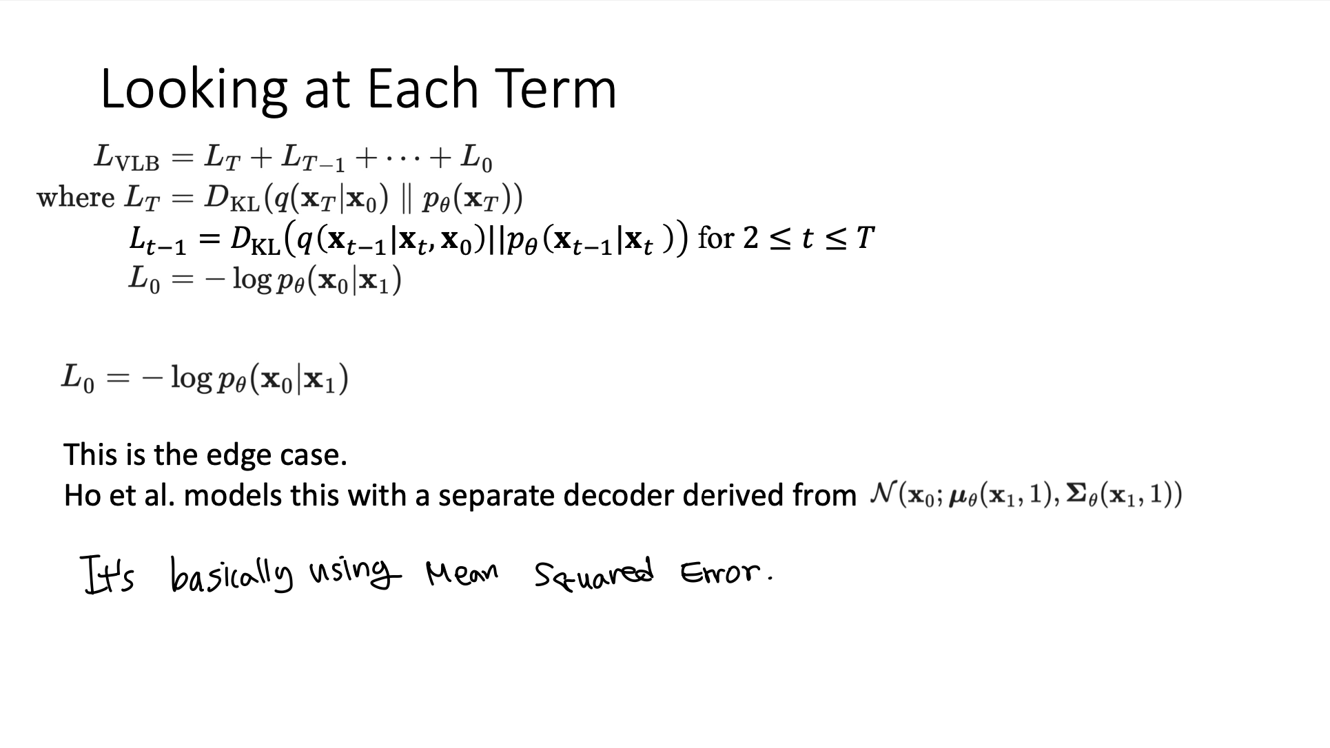
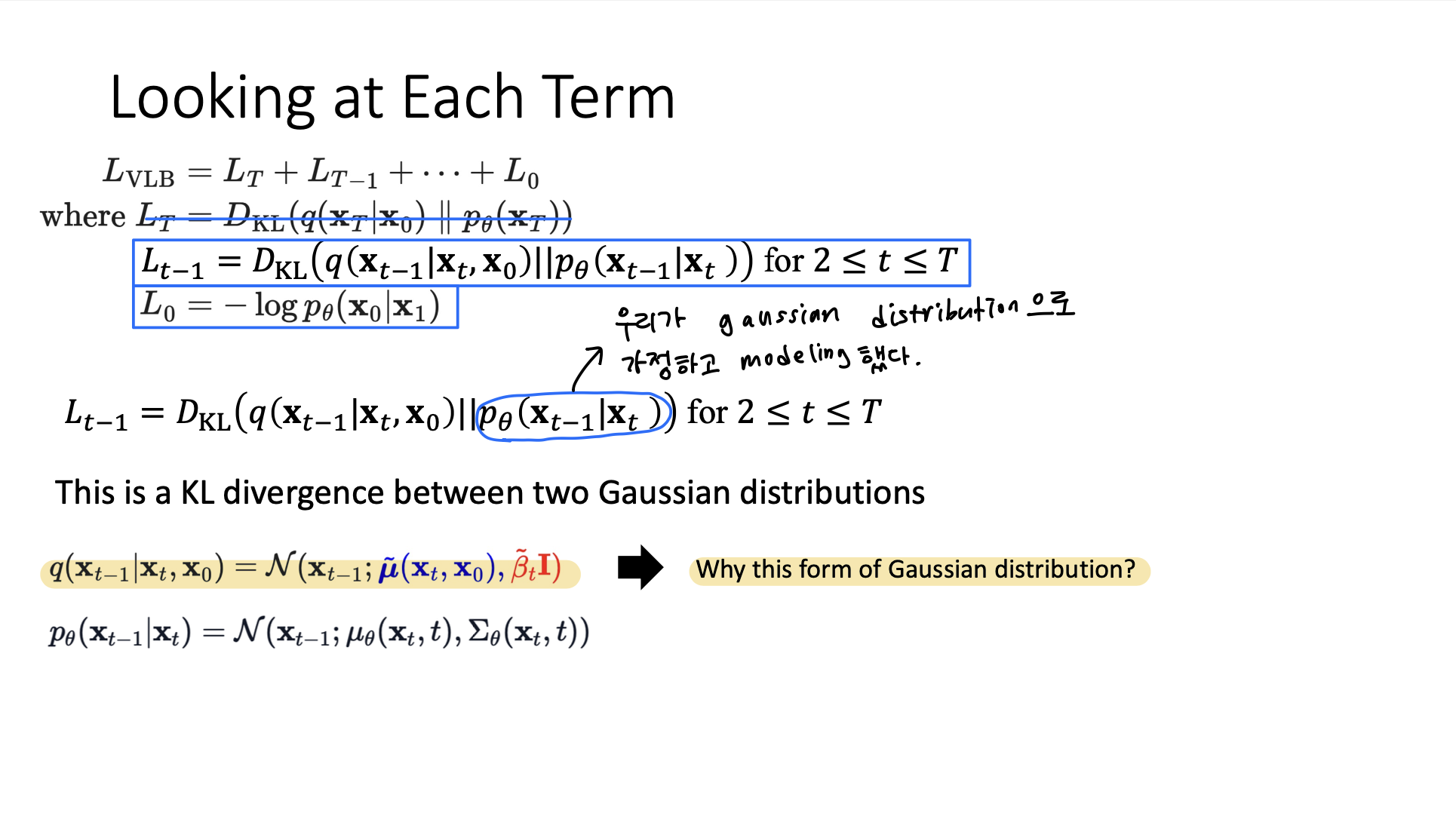
• 둘 다 gaussian이면 analytically tractable하므로 둘 다 gaussian이길 바란 것이고 실제로 gaussian이다.

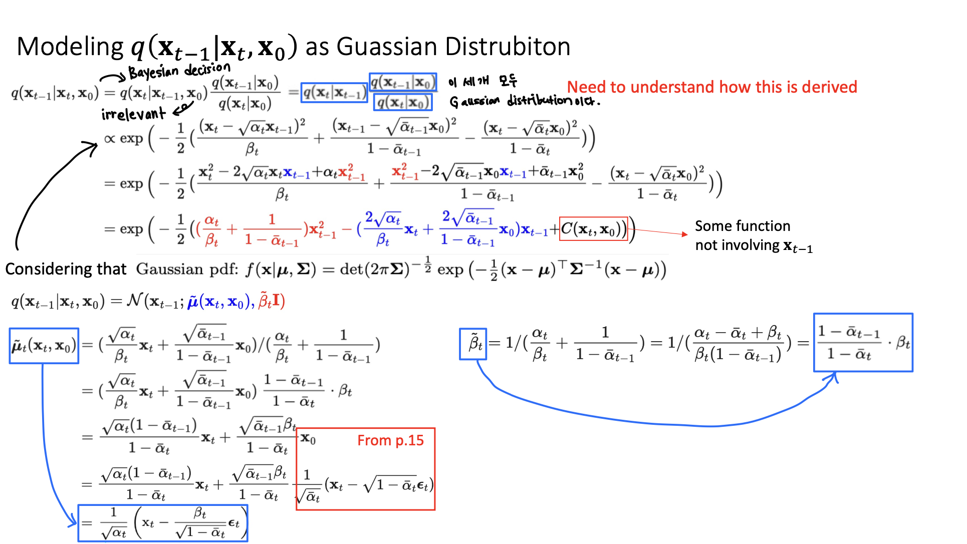
🔗 Modeling q($x_{t-1}$|$x_t$,$x_0$)

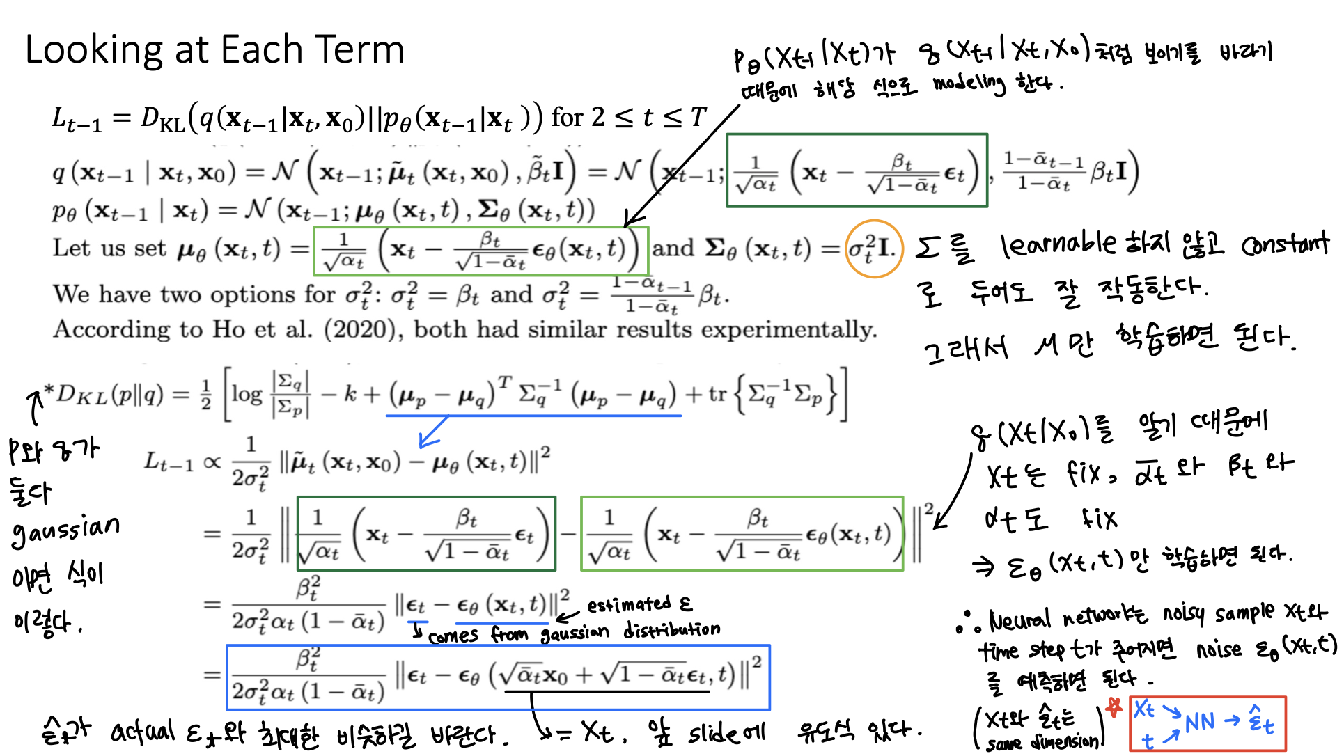
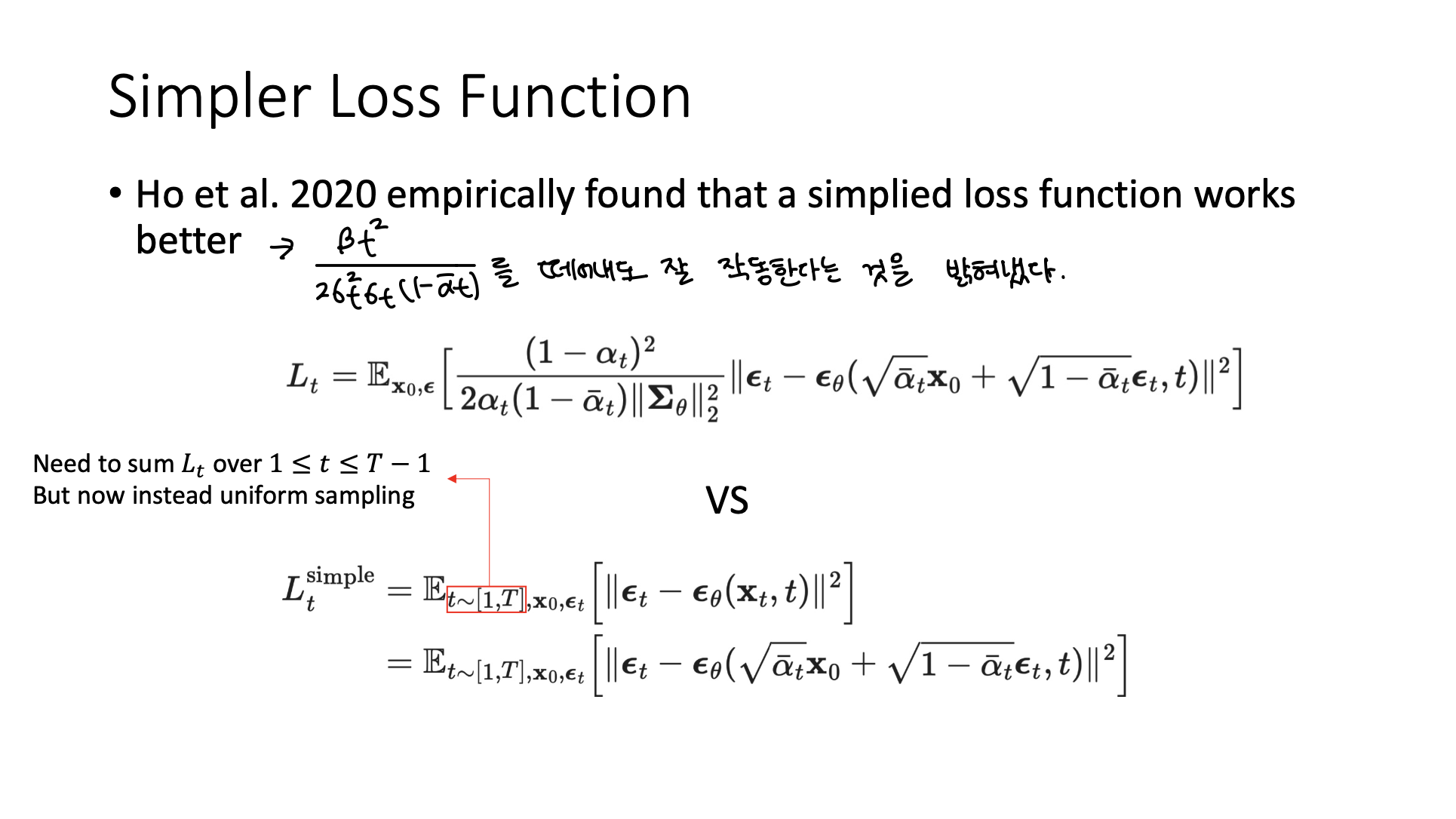
🔗 Simpler Loss Function

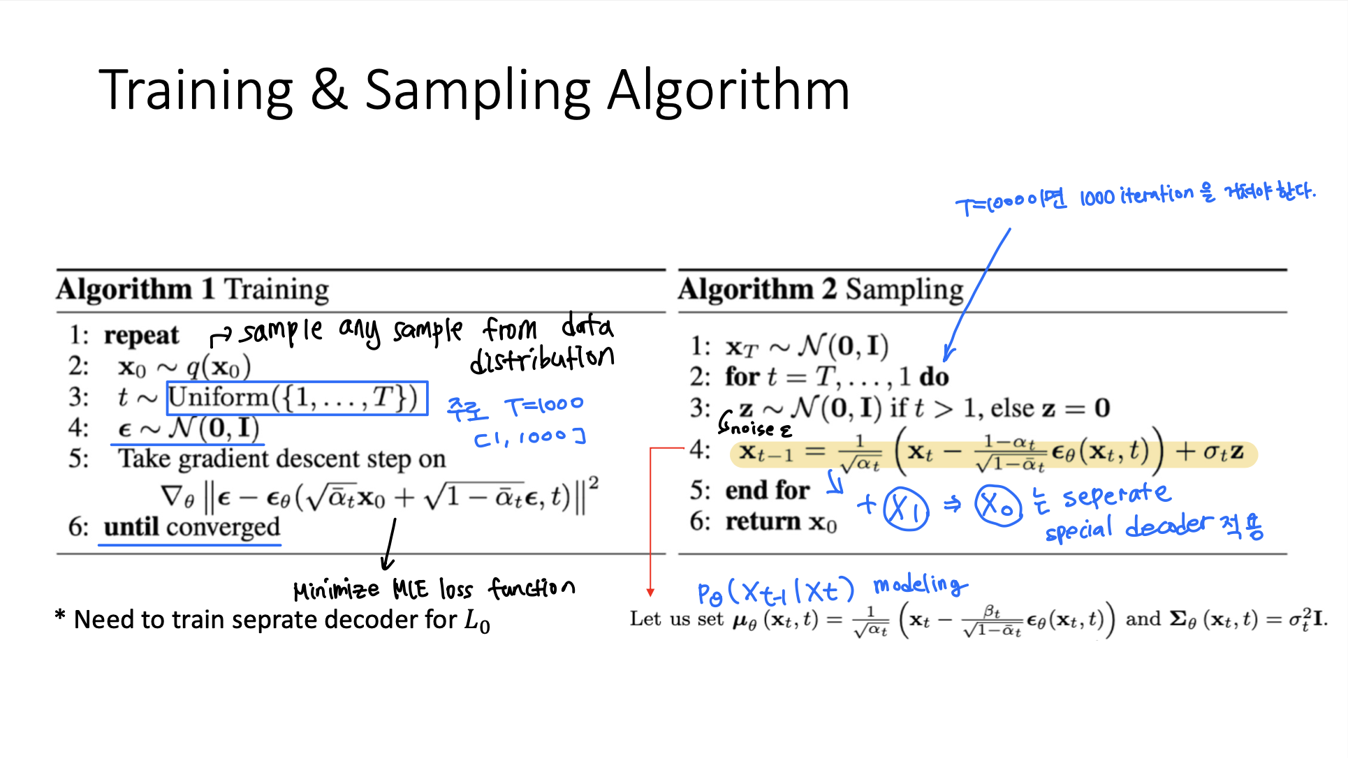
Training & Sampling Algorithm

Generation Samples

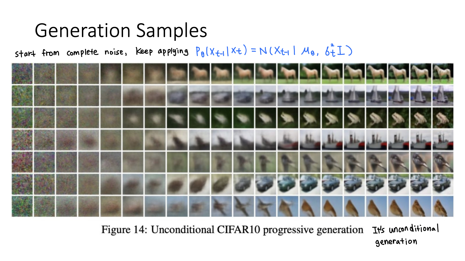
• Unconditional generation

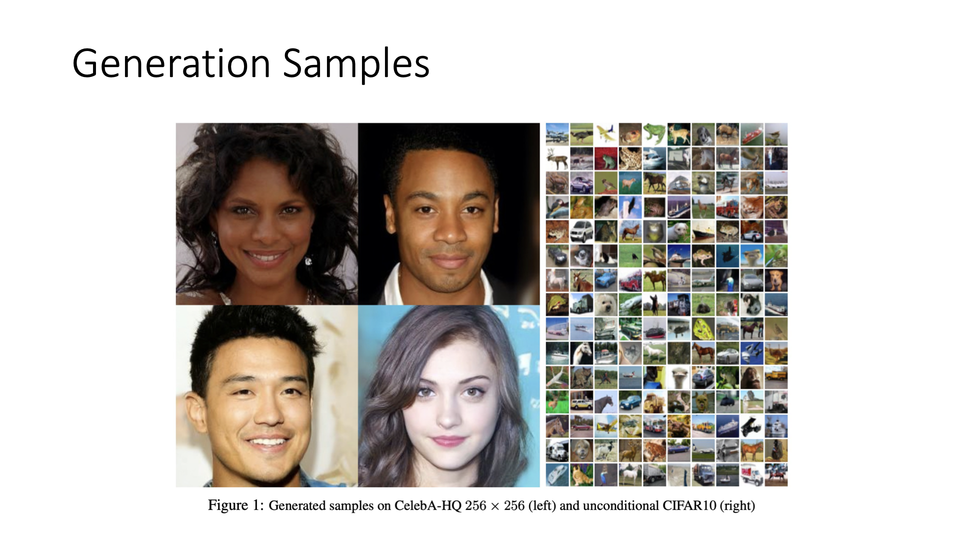
• Diffusion model의 좋은 점은 high dimensional data에도 잘 동작한다는 것이다.

GAN model은 generate한 image가 high quality를 가진다는 장점이 있지만, mode collapse에 빠질 수 있고 training이 unstable하다는 단점이 있다.
Diffusion model은 GAN model의 이 두가지 한계를 극복했다. Stable한 optimization process를 가지며 다양한 sample을 generate한다. 그리고 mode collapse에 빠지지 않는다.
하지만 diffusion model은 느리다는 단점이 있다. T=1000일때, 1개의 sample을 만들기 위해서 for loop을 1000번 돌아야한다. 매우 매우 느리다.

Improved DDPM

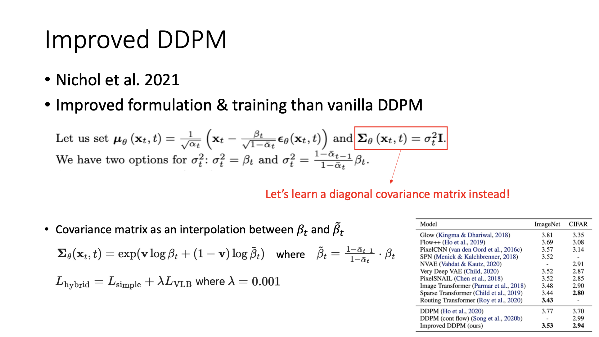
• Covariance matrix Σ를 constant로 취급하지 않고 학습한다.
• Covariance matrix를 $β_t$와 $β_t$ hat간의 interpolation으로 modeling한다.
• 이를 통해 image quality 등의 측면에서 더 좋은 성능을 보였다.

Generalized DDPM (DDIM)

💡 배경

• Drawback of DDPM : DDPM은 generation process가 너무 느리다.

➡️ DDPM을 non-Markovian으로 generalized하면 2가지 장점이 있다.

• Deterministic sampling (DDIM)을 수행할 수 있다.
  • Original DDPM에서는, $X_T$에서 시작하여 매 single reverse process마다 noise를 주입했기 때문에, 매번 다른 sample이 generate되었다.
  • 하지만 DDIM을 사용하면, non-Markovian sampling process를 사용하여, $X_T$에서 시작하여 항상 같은 sample을 generate할 수 있다.
• Sampling할 때 multiple steps를 취할 수 있다. (accelerated sampling)

Core idea

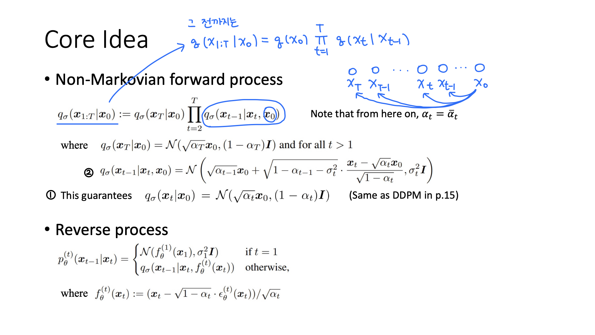
• Forward process에서 Markovian을 가정하지 않아, 이제 forward process가 아니라 모든 것이 $x_0$에 dependency가 있다.
• ① Markovian assumtion을 깨도 original DDPM과 같은 $q_σ$($x_t$ | $x_0$)에 도달하기 위해 ② 함수를 이렇게 두었다.

🔗 Properties of Generalized DDPM

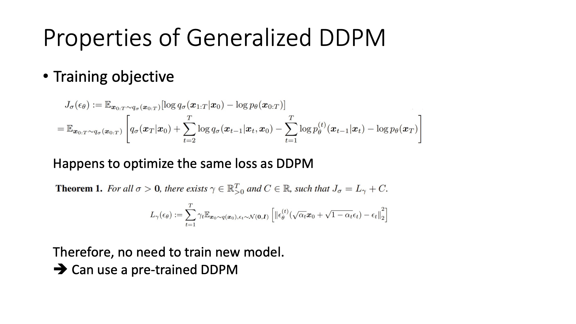
• DDPM과 같은 loss를 optimize 하므로 새로운 model을 training할 필요 없이 pre-trained DDPM을 사용할 수 있다.

Sampling Process

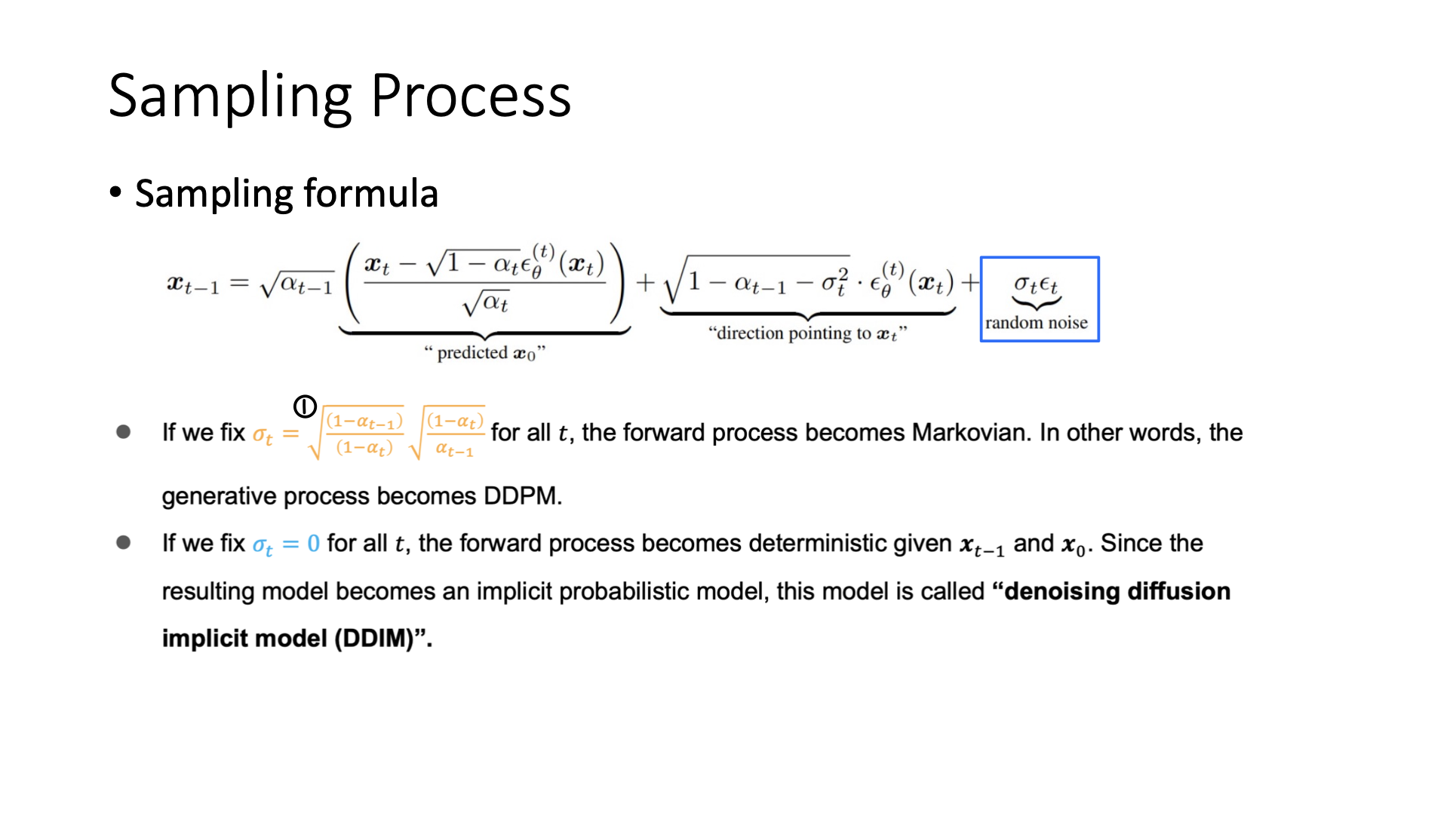
• Sampling process의 randomness를 조절할 수 있다.
  • Random noise $σ_t$ = 0 : DDIM이 되어 deterministic sampling을 하게 된다.
  • Random noise $σ_t$ = ① : DDPM이 된다. Forward process가 Markovian assumption을 하게 된다.

🔗 Accelerated Sampling

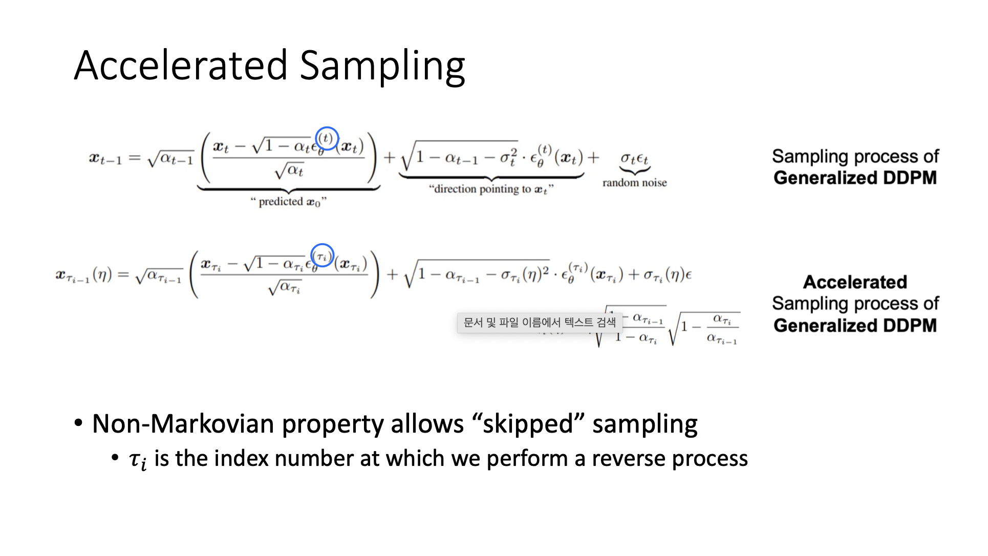
• 다른 time step으로 이동할 수 있다.

Comparison

🔗 DDPM vs DDIM

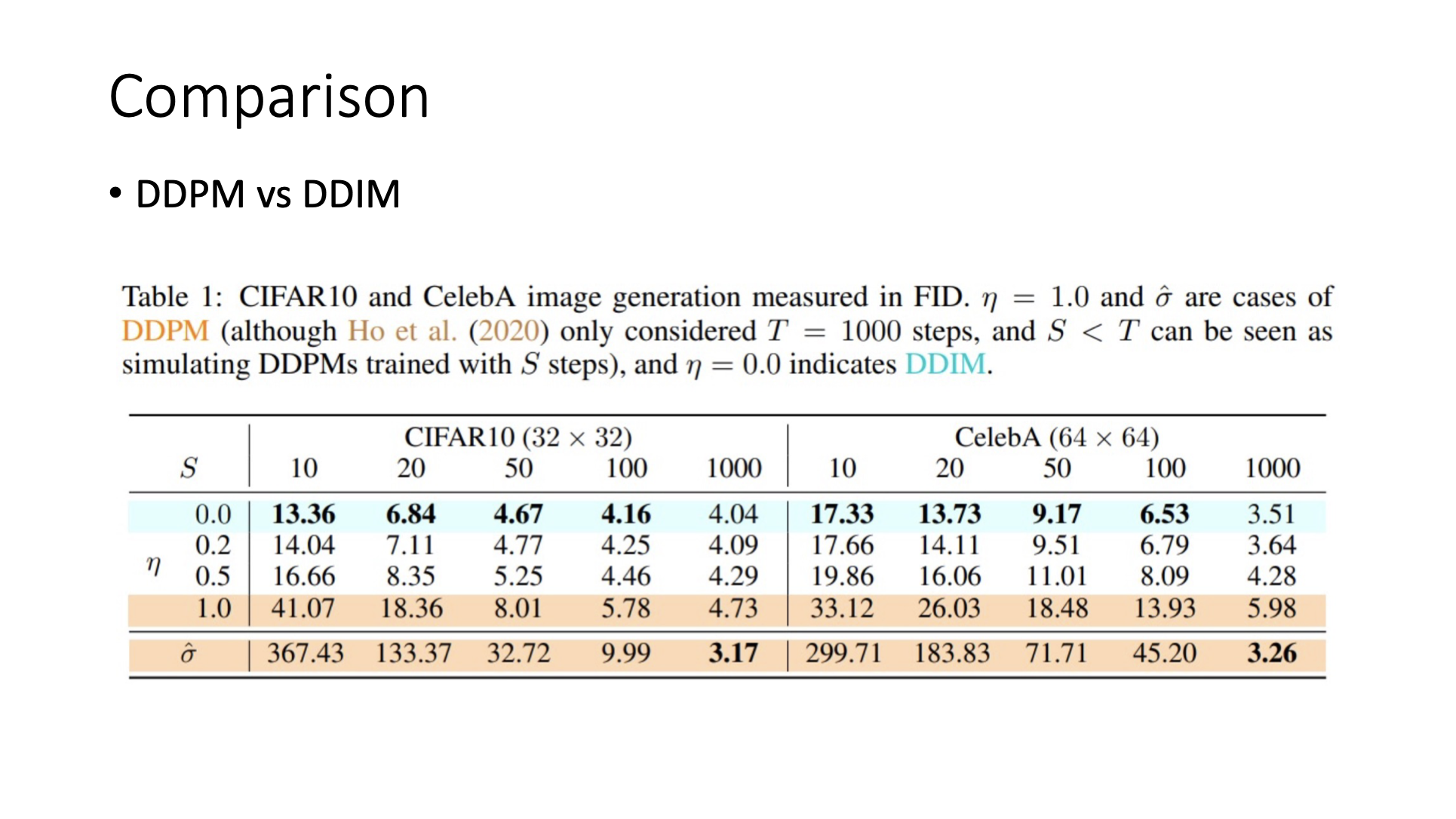
• DDPM은 T가 줄면 급격하게 FID가 증가한다.
• DDIM은 T가 1000에서 10으로 줄어도 FID가 3배정도만 증가한다. 그리고 T=100일때도 성능이 좋다.
• T=1000일때를 보면 DDPM이 살짝 더 quality가 좋긴 하다.

Guided Sampling

• Conditional sampling이라고 한다.
• Conditional sampling을 하는 두 가지 방법이 있다.
  1. Classifier-guide sampling
  2. Classifier-free sampling

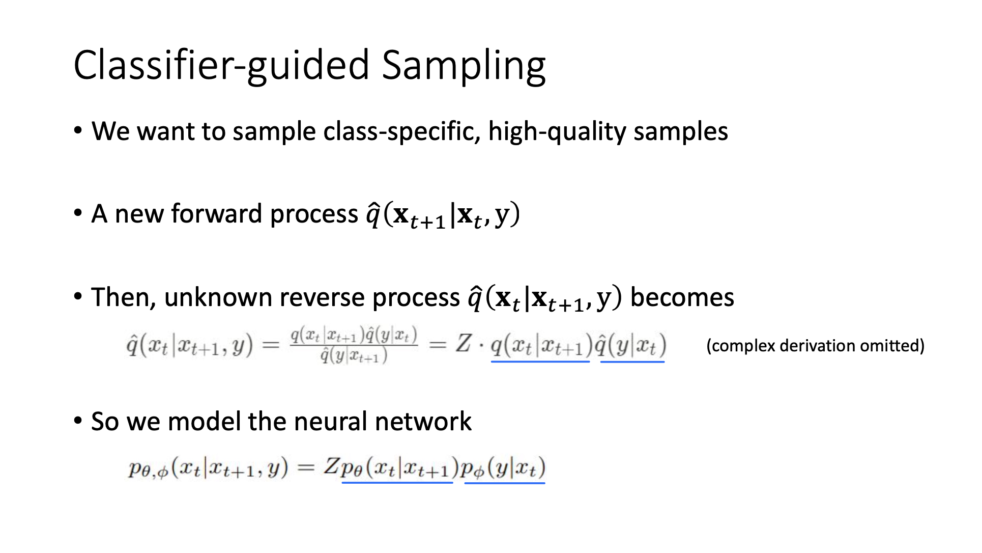
Classifier-guided Sampling

• Class-specific, high-quality samples를 sample하고싶다.

• A new forward process : previous $x_t$뿐만 아니라 preference class y도 conditioning한다.

  • y는 one-hot representation이나 특정 class를 represent하는 token이다.

• Reverse process를 original reverse process와 classifier 두 part로 나눌 수 있다. 임의의 noise level과 함께 noise sample이 주어지면, 이 noise sample을 특정 class로 분류하는 classifier가 필요하다.

• 그래서 이미 pre-trained된 $p_θ$를 classifier와 결합하여 재사용한다. 그리고 원하는대로 sampling한다.

  • 이렇게 train하면 original DDPM을 재사용할 수 있고, 원하는 특정 class를 sampling하도록 sampling process를 guide할 수 있다.
  • 예를 들어 오직 dog class만, 혹은 car class만 원하는대로 sampling할 수 있다.
  • 하지만 seperate classifier가 필요하다.

🔗 Conditional Reverse Process

어떻게 이게 동작하는지를 보여준다.

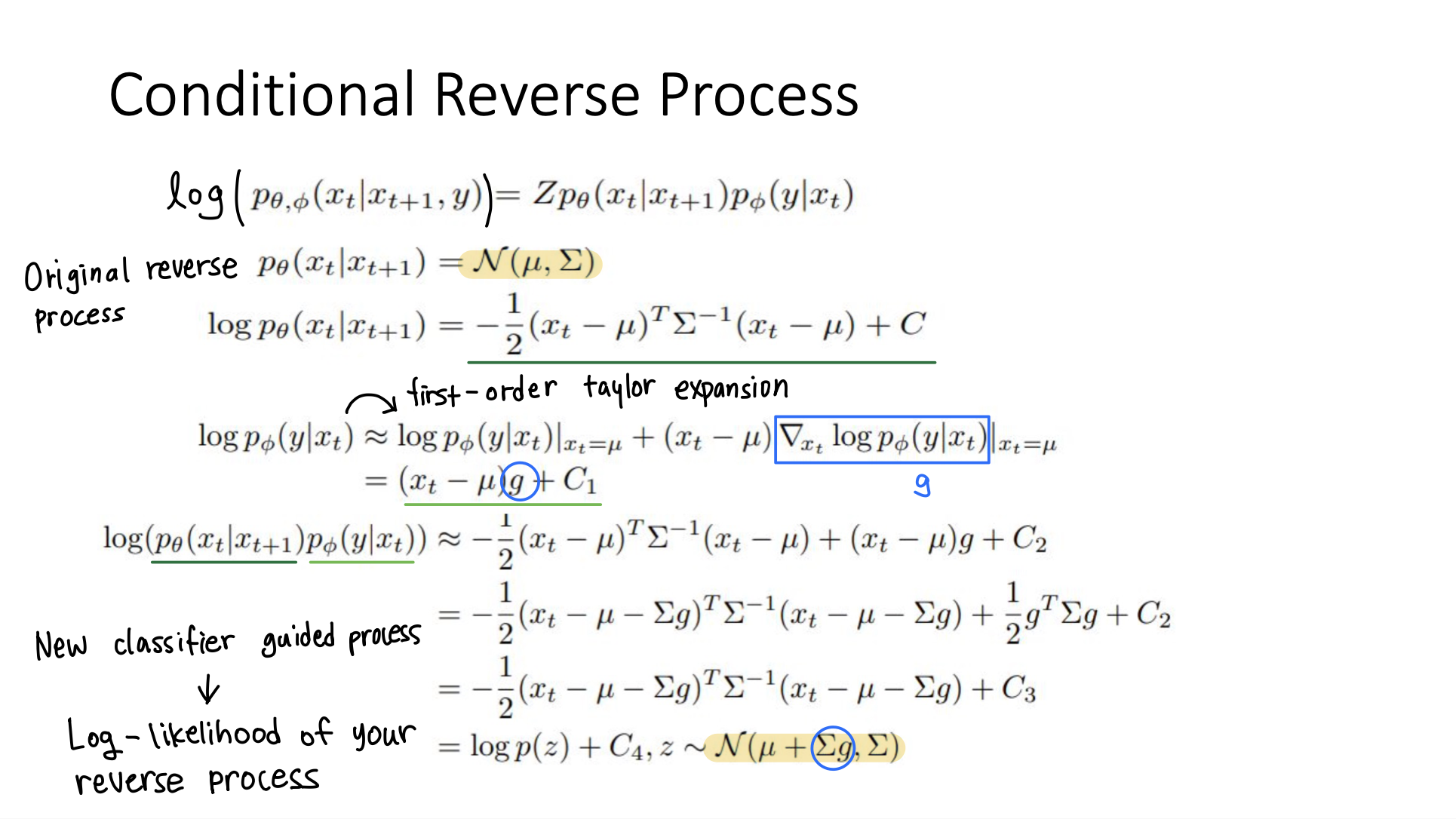
• 이렇게 함으로써 이제 sampling process가 classifier의 gradient에 의해 guide된다. 그래서 classifier가 noisy sample $x_t$를 원하는 class로 분류할 가능성이 높은 영역으로 reverse process를 조정한다.

🔗 Classifier-guided Sampling Algorithm

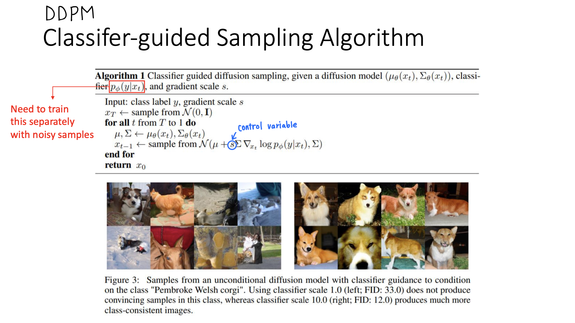
• s control variable : 너의 reverse process를 preferred class의 image로 generate하도록 하기 위해 얼마나 guide할 것인가?
  • s가 높아질 수록 class-consistant한 image가 생성됨을 볼 수 있다.
• 단점 : 여러 다른 level의 noise의 noisy sample들에 대해 train시킨 seperate classifier가 필요하다.

이 모든 공식들은 DDPM에서만 사용될 수 있다. 이 공식들을 바로 DDIM으로 적용시킬 수 없다.

Classifier-guided DDIM

DDIM을 위해서는 특별한 조취가 필요하다.

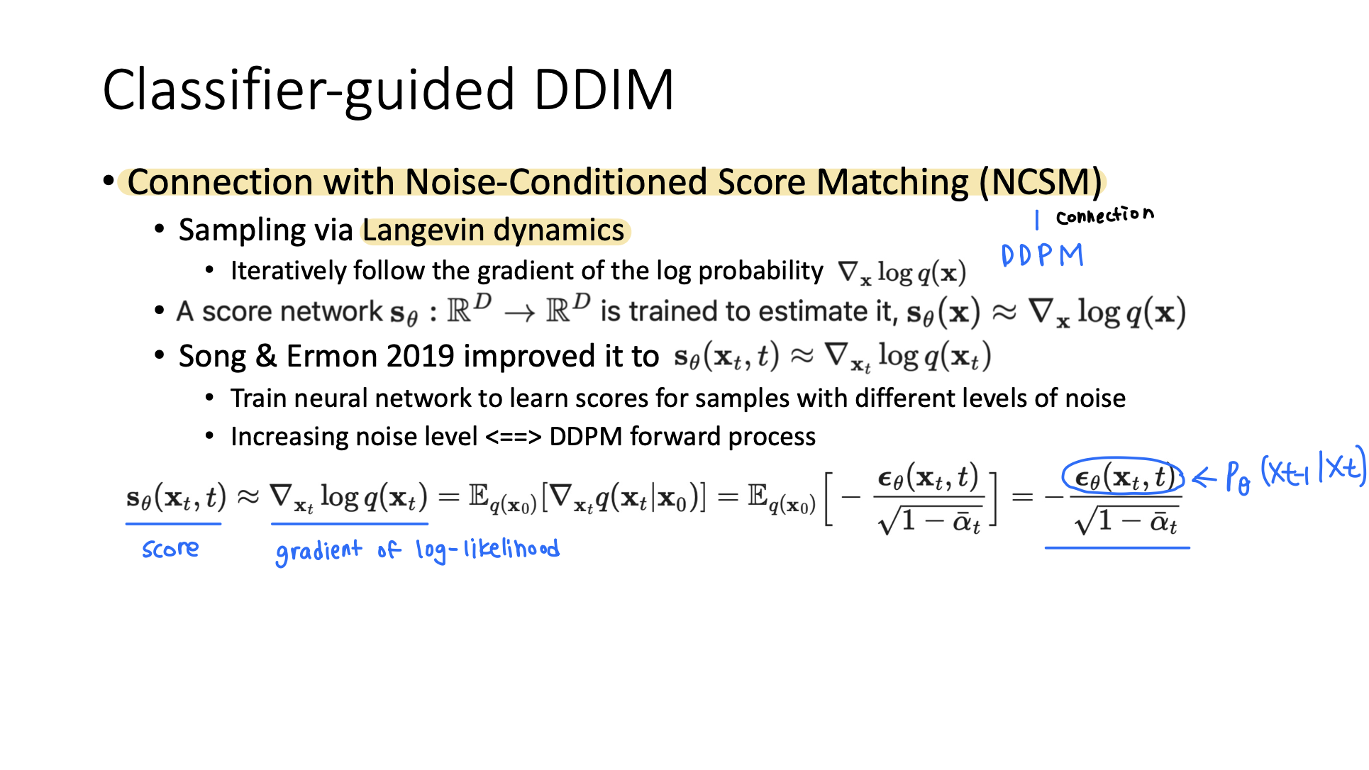
• DDPM과 Langevin dynamics를 기반으로 하는 NCSM간의 connection을 만들어야한다.
  • Langevin dynamics에서는 gradient of log-likelihood of your data distribution을 approximate하는 score로부터 sample을 sampling한다.
  • 여기서 gradient of log-likelihood가 어떻게 $p_θ$($x_{t-1}$|$x_t$}로부터 학습한 $ε_θ$($x_t$,t)로 보여질 수 있는지 그 connection을 만들어준다.
  • Whole DDPM reverse process는 ε를 학습하는 것인데, 이 ε를 학습함으로써, gradient of log-likelihood를 학습할 수 있고, 이 gradient of log-likelihood는 Langevin dynamics를 이용하여 realistic sample을 sampling하는 데에 사용될 수 있다. 이렇게 connection을 만들어준 것이다.

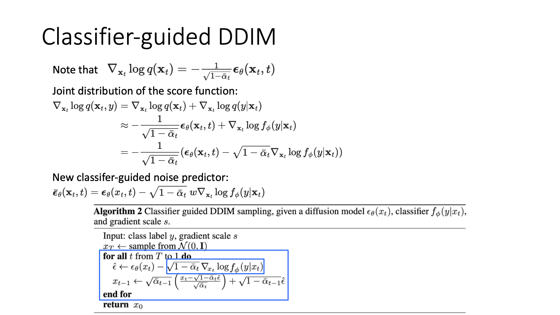
• 이렇게 만들어준 connection으로부터 새로운 sampling process를 도출할 수 있다.

➡️ Classifier-guidance가 DDPM뿐만 아니라 DDIM에도 사용될 수 있다.

Classifier-free Guidance

Gradient of log-likelihood를 이용해 classifier-guidance 방식으로 ε를 estimate하는 이 모든 concept이 classifier-free guidance에도 사용된다.
Reverse process에서 gradient of log-likelihood와 ε간의 connection을 만들 수 있다. 이를 통해 pretrained classifier가 따로 없어도 원하는 class의 sample을 generate하도록 conditioned할 수 있다.

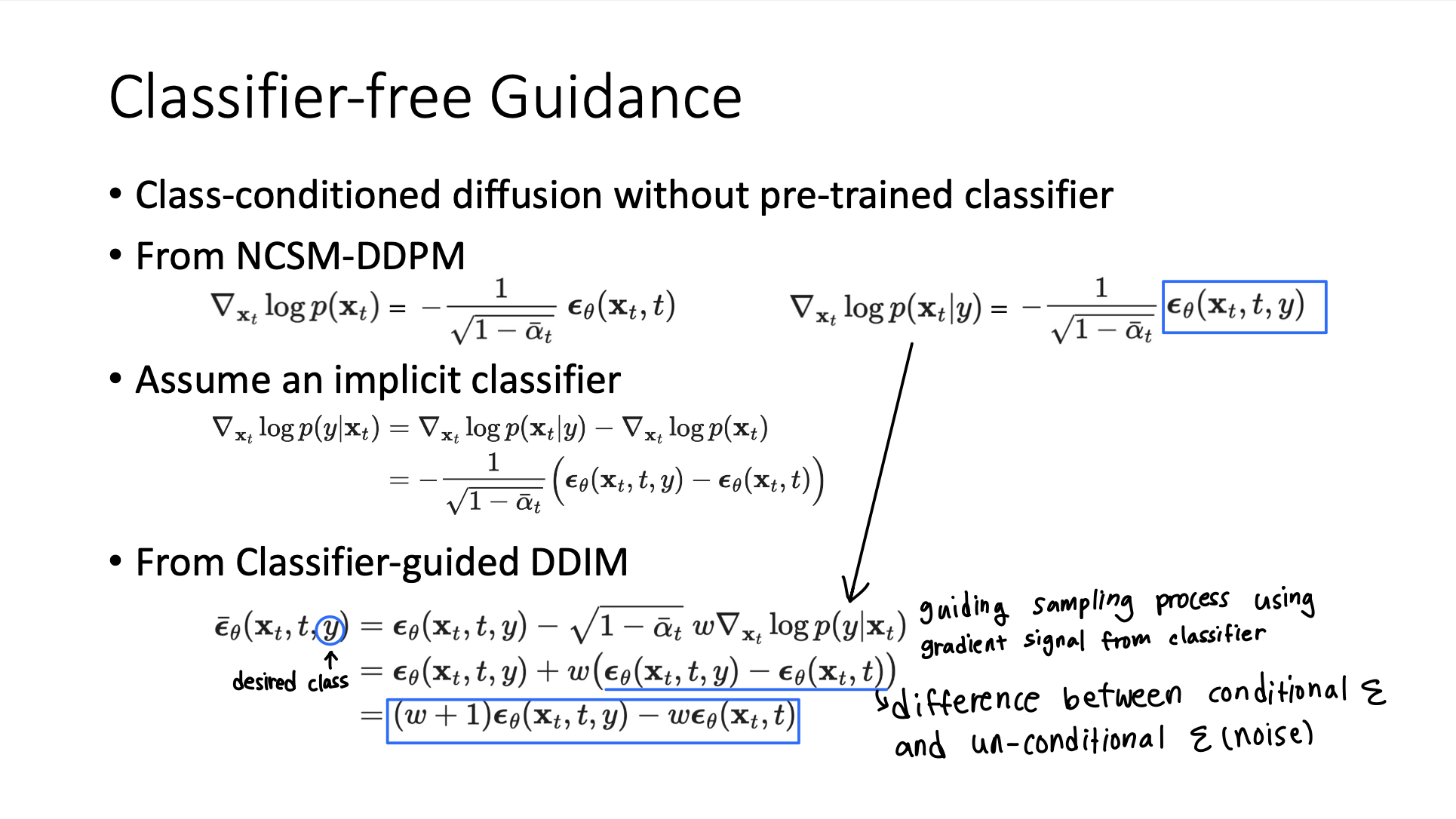
• $x_t$, t, y로 결정되는 single neural network $ε_θ$($x_t$,t,y)를 training함으로써, predicted noise를 class-conditional ε와 class-unconditional ε간의 linear combination으로 볼 수 있다. 그리고 이렇게 linear combination으로 사용해서 sampling process를 desired class의 sample을 generate하도록 guide할 수 있다.

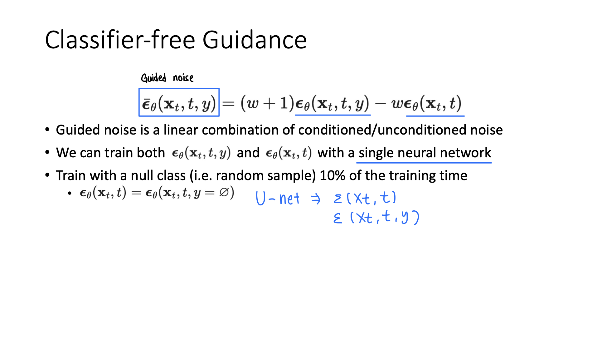
• Reverse process(generate)를 할 때 원하는 sample을 generate하게 하기 위해 $ε_θ$($x_t$,t,y)와 $ε_θ$($x_t$,t) 간의 linear combination을 사용할 수 있다.

• $ε_θ$($x_t$,t,y)와 $ε_θ$($x_t$,t)를 둘 다 single neural network로 train할 수 있다.

  • Trick : 가끔은 null class(random sample)로 train을 한다.
  • 이 single neural network로는 autoencoder처럼 생긴 U-net을 쓴다.

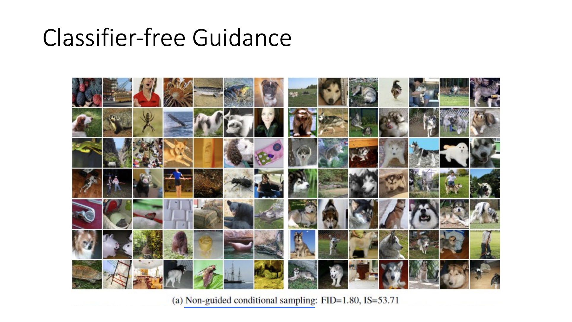
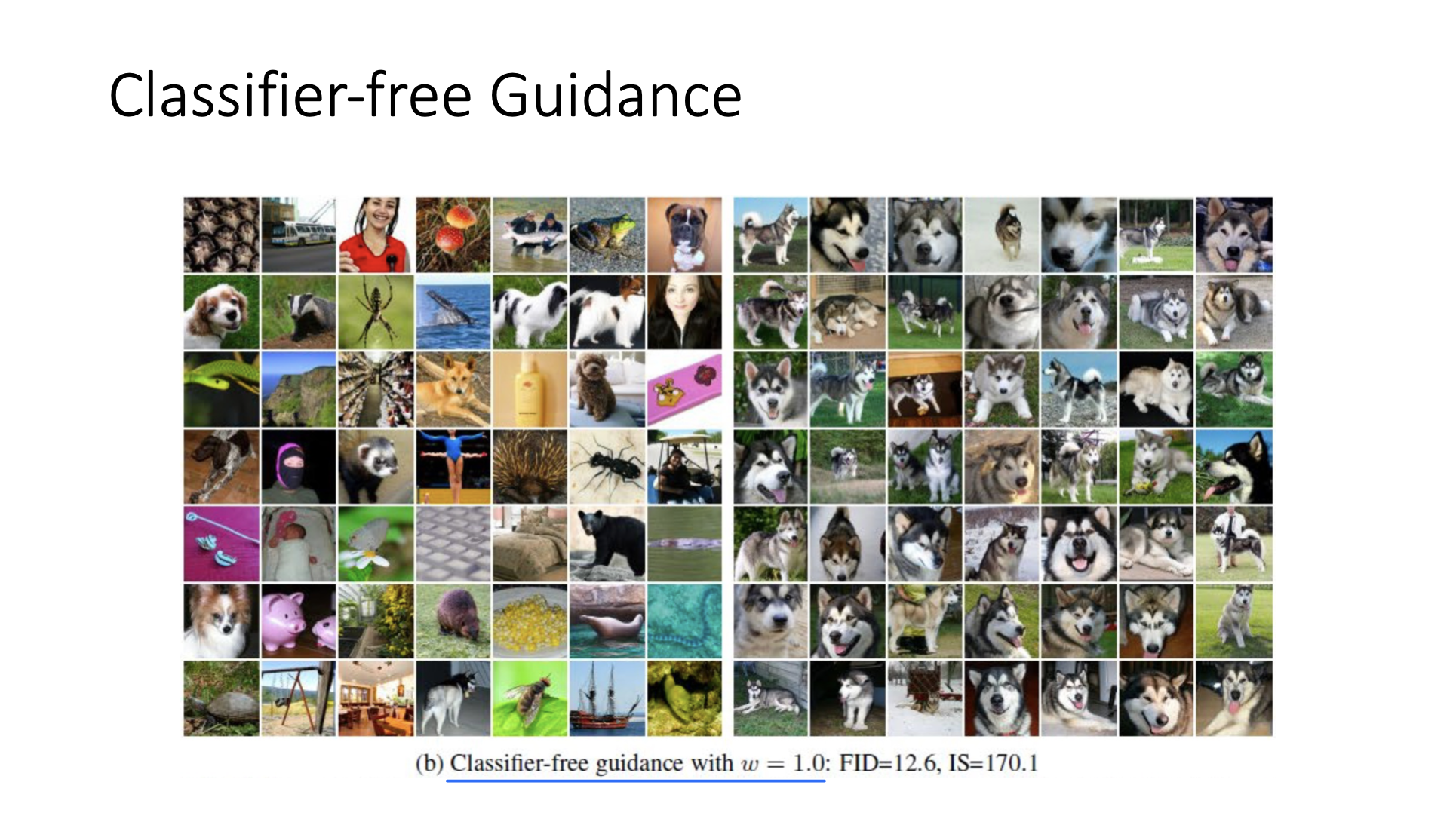
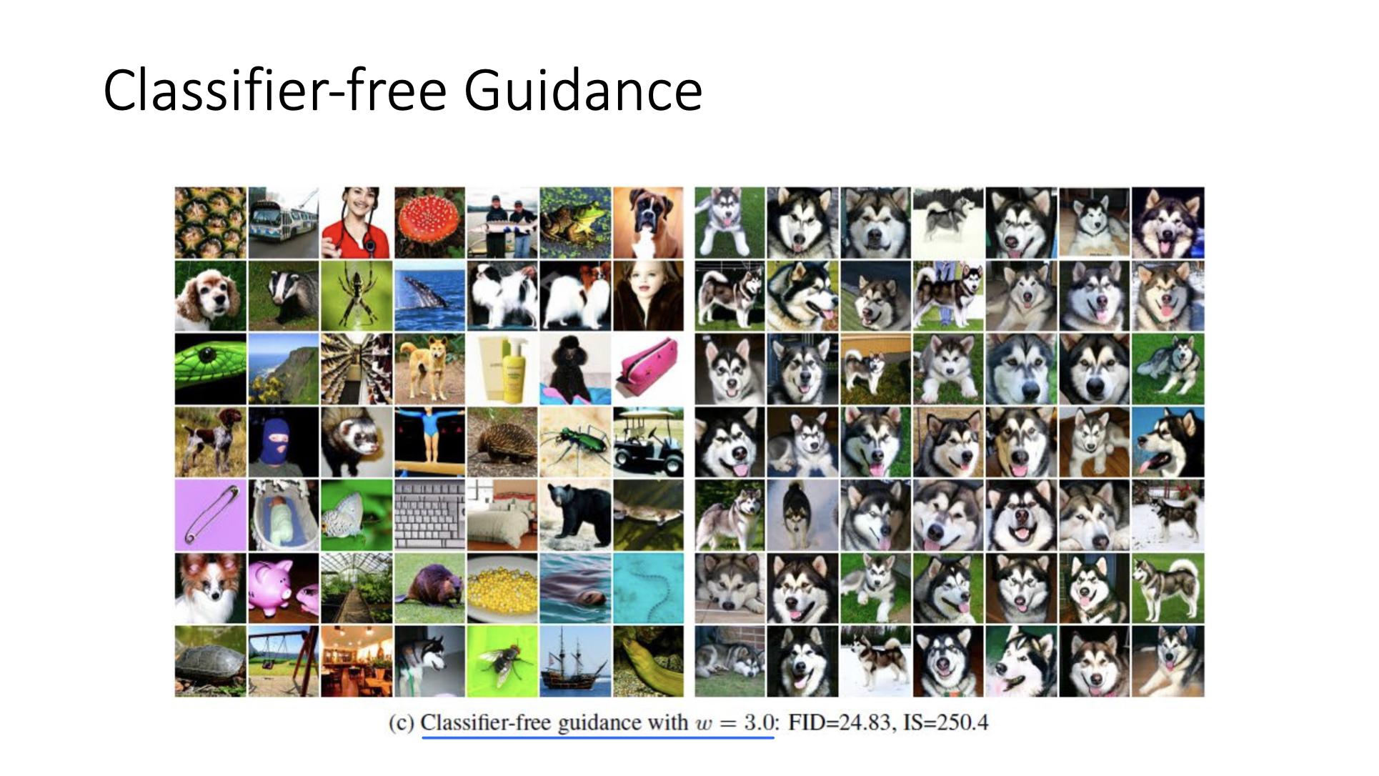
• w term을 reverse process를 control하는 데 사용한다.
  • w가 높아질 수록 원하는 class의 sample을 생성하며, diversity를 잃어간다.
    • w가 높아질수록 diffusion model을 매우 dog처럼 생긴 sample만 generate하도록 guide하기 때문에 매우 좁은 범위의 sample들에만 집중한다.

Diffusion을 위해 하나의 neural network만 train하고 이를 이용해서 preferred class의 sample을 conditionally generate할 수 있다. 그래서 classifier-free guidance라고 불린다.

✔️ Variational Lower Bound

Reference

• AI504: Programming for AI Lecture at KAIST AI