Week 14: GNN
Today class consists of three things.
1. We will Make Graph Convolution Equation.
1-1. We will make graph by using networx libary.
1-2. by using Adjacency Matrix, Node index and Node embedding vector from graph, We will follow the aggregation and combination step in Graph Convolution Equation.
1-3. Finally We will make GCN layer
2. We will make node classification in Cora dataset.
2-1. Cora dataset Information
2-2. Implement GCN model with Cora dataset
2-3. Visualize node embedding
3. (DIY) Run the Graph classification on the Collab Dataset
3-1. I will introduce some brief information about the code and pytorch geometric.
If you have any questions, feel free to ask
- E-Mail Address : pacesun@kaist.ac.kr
- Code made by Seongjun Yang at KAIST GSAI Edlab
Prelims
!pip install ipdbLooking in indexes: https://pypi.org/simple, https://us-python.pkg.dev/colab-wheels/public/simple/
Collecting ipdb
Downloading ipdb-0.13.13-py3-none-any.whl (12 kB)
Collecting ipython>=7.31.1
Downloading ipython-8.11.0-py3-none-any.whl (793 kB)
[2K [90m━━━━━━━━━━━━━━━━━━━━━━━━━━━━━━━━━━━━━━[0m [32m793.3/793.3 KB[0m [31m11.7 MB/s[0m eta [36m0:00:00[0m
[?25hRequirement already satisfied: tomli in /usr/local/lib/python3.9/dist-packages (from ipdb) (2.0.1)
Requirement already satisfied: decorator in /usr/local/lib/python3.9/dist-packages (from ipdb) (4.4.2)
Requirement already satisfied: pickleshare in /usr/local/lib/python3.9/dist-packages (from ipython>=7.31.1->ipdb) (0.7.5)
Collecting prompt-toolkit!=3.0.37,<3.1.0,>=3.0.30
Downloading prompt_toolkit-3.0.38-py3-none-any.whl (385 kB)
[2K [90m━━━━━━━━━━━━━━━━━━━━━━━━━━━━━━━━━━━━━━[0m [32m385.8/385.8 KB[0m [31m25.9 MB/s[0m eta [36m0:00:00[0m
[?25hCollecting jedi>=0.16
Downloading jedi-0.18.2-py2.py3-none-any.whl (1.6 MB)
[2K [90m━━━━━━━━━━━━━━━━━━━━━━━━━━━━━━━━━━━━━━━━[0m [32m1.6/1.6 MB[0m [31m46.9 MB/s[0m eta [36m0:00:00[0m
[?25hRequirement already satisfied: backcall in /usr/local/lib/python3.9/dist-packages (from ipython>=7.31.1->ipdb) (0.2.0)
Requirement already satisfied: pygments>=2.4.0 in /usr/local/lib/python3.9/dist-packages (from ipython>=7.31.1->ipdb) (2.14.0)
Collecting stack-data
Downloading stack_data-0.6.2-py3-none-any.whl (24 kB)
Requirement already satisfied: pexpect>4.3 in /usr/local/lib/python3.9/dist-packages (from ipython>=7.31.1->ipdb) (4.8.0)
Collecting matplotlib-inline
Downloading matplotlib_inline-0.1.6-py3-none-any.whl (9.4 kB)
Requirement already satisfied: traitlets>=5 in /usr/local/lib/python3.9/dist-packages (from ipython>=7.31.1->ipdb) (5.7.1)
Requirement already satisfied: parso<0.9.0,>=0.8.0 in /usr/local/lib/python3.9/dist-packages (from jedi>=0.16->ipython>=7.31.1->ipdb) (0.8.3)
Requirement already satisfied: ptyprocess>=0.5 in /usr/local/lib/python3.9/dist-packages (from pexpect>4.3->ipython>=7.31.1->ipdb) (0.7.0)
Requirement already satisfied: wcwidth in /usr/local/lib/python3.9/dist-packages (from prompt-toolkit!=3.0.37,<3.1.0,>=3.0.30->ipython>=7.31.1->ipdb) (0.2.6)
Collecting asttokens>=2.1.0
Downloading asttokens-2.2.1-py2.py3-none-any.whl (26 kB)
Collecting executing>=1.2.0
Downloading executing-1.2.0-py2.py3-none-any.whl (24 kB)
Collecting pure-eval
Downloading pure_eval-0.2.2-py3-none-any.whl (11 kB)
Requirement already satisfied: six in /usr/local/lib/python3.9/dist-packages (from asttokens>=2.1.0->stack-data->ipython>=7.31.1->ipdb) (1.16.0)
Installing collected packages: pure-eval, executing, prompt-toolkit, matplotlib-inline, jedi, asttokens, stack-data, ipython, ipdb
Attempting uninstall: prompt-toolkit
Found existing installation: prompt-toolkit 2.0.10
Uninstalling prompt-toolkit-2.0.10:
Successfully uninstalled prompt-toolkit-2.0.10
Attempting uninstall: ipython
Found existing installation: ipython 7.9.0
Uninstalling ipython-7.9.0:
Successfully uninstalled ipython-7.9.0
[31mERROR: pip's dependency resolver does not currently take into account all the packages that are installed. This behaviour is the source of the following dependency conflicts.
google-colab 1.0.0 requires ipython~=7.9.0, but you have ipython 8.11.0 which is incompatible.[0m[31m
[0mSuccessfully installed asttokens-2.2.1 executing-1.2.0 ipdb-0.13.13 ipython-8.11.0 jedi-0.18.2 matplotlib-inline-0.1.6 prompt-toolkit-3.0.38 pure-eval-0.2.2 stack-data-0.6.2!pip install networkxLooking in indexes: https://pypi.org/simple, https://us-python.pkg.dev/colab-wheels/public/simple/
Requirement already satisfied: networkx in /usr/local/lib/python3.9/dist-packages (3.0)import ipdb
import torch
import networkx as nx
import numpy as np
from sklearn.manifold import TSNE
import matplotlib.pyplot as plt
from scipy.linalg import fractional_matrix_power
import warnings
warnings.filterwarnings("ignore", category=UserWarning)
device = torch.device("cuda:0" if torch.cuda.is_available() else "cpu")1. Make Graph Convolution Equation
1) Initialize the Graph G
By using networkx library, you can do research in graph or network easily.
So, in the Graph Convolution Equation, I'll use networkx libary.
#1. Initialize the graph
G = nx.Graph(name='G')G<networkx.classes.graph.Graph at 0x7fa9bc302e20>#2. Create nodes
#In this class, we will make graph that consist of 6 nodes.
#Each node is assigned node feature which corresponds to the node name
for i in range(1,7):
G.add_node(i, name=i)#Define the edges and the edges to the graph
edges = [(1,2), (1,3), (2,4), (2,5), (3,4), (3,6) ]
G.add_edges_from(edges)#Inspect the node features
print('\nGraph Nodes: ', G.nodes.data())Graph Nodes: [(1, {'name': 1}), (2, {'name': 2}), (3, {'name': 3}), (4, {'name': 4}), (5, {'name': 5}), (6, {'name': 6})]#Plot the graph
nx.draw(G, with_labels=True, font_weight='bold')
plt.show()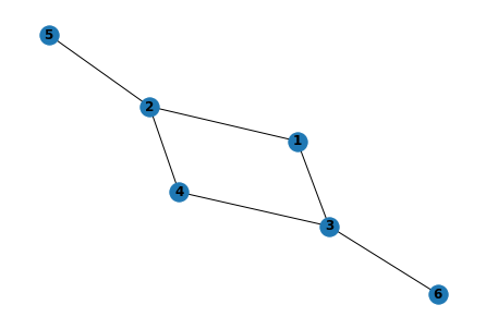
Inserting Adjacency Matrix to forward pass
# Adjacency Matrix
nx.attr_matrix(G, node_attr='name')
(array([[0., 1., 1., 0., 0., 0.],
[1., 0., 0., 1., 1., 0.],
[1., 0., 0., 1., 0., 1.],
[0., 1., 1., 0., 0., 0.],
[0., 1., 0., 0., 0., 0.],
[0., 0., 1., 0., 0., 0.]]), [1, 2, 3, 4, 5, 6])#Get the Adjacency Matrix (A) and Node Features Matrix (X) as numpy array
A = np.array(nx.attr_matrix(G, node_attr='name')[0]) # Converting for getting numpy Adjacency Matrix (A)
X = np.array(nx.attr_matrix(G, node_attr='name')[1]) # Converting for getting numpy Node Features Matrix (X)
X = np.expand_dims(X,axis=1) # Make [6, 1] numpy Node Features Matrix (X)print('Shape of A: ', A.shape) # [6, 6] matrixShape of A: (6, 6)print('\nShape of X: ', X.shape) # [6, 1] matrixShape of X: (6, 1)print('\nAdjacency Matrix (A):\n', A)Adjacency Matrix (A):
[[0. 1. 1. 0. 0. 0.]
[1. 0. 0. 1. 1. 0.]
[1. 0. 0. 1. 0. 1.]
[0. 1. 1. 0. 0. 0.]
[0. 1. 0. 0. 0. 0.]
[0. 0. 1. 0. 0. 0.]]print('\nNode Features Matrix (X):\n', X)Node Features Matrix (X):
[[1]
[2]
[3]
[4]
[5]
[6]]#Dot product Adjacency Matrix (A) and Node Features (X)
AX = np.dot(A,X) # AX
print("Dot product of A and X (AX):\n", AX)Dot product of A and X (AX):
[[ 5.]
[10.]
[11.]
[ 5.]
[ 2.]
[ 3.]]Question : Is this the node representations H?
No, A*X is just neighbor aggregation.
We need the combination step!
Add Self-Loops and Normalize Adjacency Matrix (A)
A' = A + I
#Add Self Loops
G_self_loops = G.copy() # A'

self_loops = []
for i in range(1, 1+ G.number_of_nodes()):
    self_loops.append((i,i))

G_self_loops.add_edges_from(self_loops) # A' = A + I
#Check the edges of G_self_loops after adding the self loops
print('Edges of G with self-loops:\n', G_self_loops.edges)
Edges of G with self-loops:
[(1, 2), (1, 3), (1, 1), (2, 4), (2, 5), (2, 2), (3, 4), (3, 6), (3, 3), (4, 4), (5, 5), (6, 6)]#Get the Adjacency Matrix (A) and Node Features Matrix (X) of added self-lopps graph
A_hat = np.array(nx.attr_matrix(G_self_loops, node_attr='name')[0]) # A' numpy Matrix
print('Adjacency Matrix of added self-loops G (A_hat):\n', A_hat)Adjacency Matrix of added self-loops G (A_hat):
[[1. 1. 1. 0. 0. 0.]
[1. 1. 0. 1. 1. 0.]
[1. 0. 1. 1. 0. 1.]
[0. 1. 1. 1. 0. 0.]
[0. 1. 0. 0. 1. 0.]
[0. 0. 1. 0. 0. 1.]]A' * X Matrix
#Calculate the dot product of A_hat and X (AX)
A_hatX = np.dot(A_hat, X)
print('A_hatX:\n', A_hatX)
A_hatX:
[[ 6.]
[12.]
[14.]
[ 9.]
[ 7.]
[ 9.]]But, there is another problem.
Scales of node features differ by the number of neighbors.
Solution : Normalization by inverse degree matrix.
D_inverse * A'
#Get the Degree Matrix of the added self-loops graph
edge_List = G_self_loops.edges()
Deg_Mat = [[i, 0] for i in G_self_loops.nodes()]

for element in edge_List:
  if element[0] != element[1]:
    Deg_Mat[element[0] - 1][1] += 1
    Deg_Mat[element[1] - 1][1] += 1
  else :
    Deg_Mat[element[0] - 1][1] += 1

print(Deg_Mat)
[[1, 3], [2, 4], [3, 4], [4, 3], [5, 2], [6, 2]]#Convert the Degree Matrix to a N x N matrix where N is the number of nodes
D = np.diag([deg for [n,deg] in Deg_Mat]) # Get degree matrix
print('Degree Matrix of added self-loops G as numpy array (D):\n', D)Degree Matrix of added self-loops G as numpy array (D):
[[3 0 0 0 0 0]
[0 4 0 0 0 0]
[0 0 4 0 0 0]
[0 0 0 3 0 0]
[0 0 0 0 2 0]
[0 0 0 0 0 2]]D_inverse
#Get the inverse of Degree Matrix (D)
D_inv = np.linalg.inv(D)
print('Inverse of D:\n', D_inv)
Inverse of D:
[[0.33333333 0. 0. 0. 0. 0. ]
[0. 0.25 0. 0. 0. 0. ]
[0. 0. 0.25 0. 0. 0. ]
[0. 0. 0. 0.33333333 0. 0. ]
[0. 0. 0. 0. 0.5 0. ]
[0. 0. 0. 0. 0. 0.5 ]]D_inverse*A'
A_hatarray([[1., 1., 1., 0., 0., 0.],
[1., 1., 0., 1., 1., 0.],
[1., 0., 1., 1., 0., 1.],
[0., 1., 1., 1., 0., 0.],
[0., 1., 0., 0., 1., 0.],
[0., 0., 1., 0., 0., 1.]])D_invA = np.dot(D_inv, A_hat)
print(D_invA)[[0.33333333 0.33333333 0.33333333 0. 0. 0. ]
[0.25 0.25 0. 0.25 0.25 0. ]
[0.25 0. 0.25 0.25 0. 0.25 ]
[0. 0.33333333 0.33333333 0.33333333 0. 0. ]
[0. 0.5 0. 0. 0.5 0. ]
[0. 0. 0.5 0. 0. 0.5 ]]D_invA'X
#Dot product of D and AX for normalization
DAX = np.dot(D_invA,X)
print('DAXW:\n', DAX)DAXW:
[[2. ]
[3. ]
[3.5]
[3. ]
[3.5]
[4.5]]Add Weights and Activation Function
#Initialize the weights
np.random.seed(12345)
n_h = 4 #number of neurons in the hidden layer
n_y = 2 #number of neurons in the output layer
W0 = np.random.randn(X.shape[1],n_h) * 0.01
W1 = np.random.randn(n_h,n_y) * 0.01
print('W0 weight:\n', W0)
print('W1 weight:\n', W1)W0 weight:
[[-0.00204708 0.00478943 -0.00519439 -0.0055573 ]]
W1 weight:
[[ 0.01965781 0.01393406]
[ 0.00092908 0.00281746]
[ 0.00769023 0.01246435]
[ 0.01007189 -0.01296221]]GCN Layer
TODO : fill ????? with proper code and run
#Implement ReLu as activation function,
#Originally, non-linear activation needed, but when I searched some material, relu is used for activate function generally.
def relu(x):
return np.maximum(0,x)
#Build GCN layer
#In this function, we implement numpy to simplify
def gcn(A,H,W):
ipdb.set_trace()
# Make a GCN Layer using the Graph Convolution Equation process so far.
# You can use np.diag, np.sum, np.linalg.inv, np.dot
I = np.identity(A.shape[0]) # create Identity Matrix of A
A_hat = A + I # add self-loop to A
D = np.diag(np.sum(A_hat, axis=0)) # create Degree Matrix of A
D_inv = np.linalg.inv(D)
D_invA = np.dot(D_inv, A_hat)
DAXW = np.dot(D_invA, H).dot(W)
return relu(DAXW)#Do forward propagation
H1 = gcn(A,X,W0) PYDEV DEBUGGER WARNING:
sys.settrace() should not be used when the debugger is being used.
This may cause the debugger to stop working correctly.
If this is needed, please check:
http://pydev.blogspot.com/2007/06/why-cant-pydev-debugger-work-with.html
to see how to restore the debug tracing back correctly.
Call Location:
File "/usr/lib/python3.9/bdb.py", line 334, in set_trace
sys.settrace(self.trace_dispatch)
> [0;32m<ipython-input-28-275b688f615f>[0m(12)[0;36mgcn[0;34m()[0m
[0;32m 11 [0;31m [0;31m# You can use np.diag, np.sum, np.linalg.inv, np.dot[0m[0;34m[0m[0;34m[0m[0m
[0m[0;32m---> 12 [0;31m [0mI[0m [0;34m=[0m [0mnp[0m[0;34m.[0m[0midentity[0m[0;34m([0m[0mA[0m[0;34m.[0m[0mshape[0m[0;34m[[0m[0;36m0[0m[0;34m][0m[0;34m)[0m [0;31m# create Identity Matrix of A[0m[0;34m[0m[0;34m[0m[0m
[0m[0;32m 13 [0;31m [0mA_hat[0m [0;34m=[0m [0mA[0m [0;34m+[0m [0mI[0m [0;31m# add self-loop to A[0m[0;34m[0m[0;34m[0m[0m
[0m
ipdb> n
> [0;32m<ipython-input-28-275b688f615f>[0m(13)[0;36mgcn[0;34m()[0m
[0;32m 12 [0;31m [0mI[0m [0;34m=[0m [0mnp[0m[0;34m.[0m[0midentity[0m[0;34m([0m[0mA[0m[0;34m.[0m[0mshape[0m[0;34m[[0m[0;36m0[0m[0;34m][0m[0;34m)[0m [0;31m# create Identity Matrix of A[0m[0;34m[0m[0;34m[0m[0m
[0m[0;32m---> 13 [0;31m [0mA_hat[0m [0;34m=[0m [0mA[0m [0;34m+[0m [0mI[0m [0;31m# add self-loop to A[0m[0;34m[0m[0;34m[0m[0m
[0m[0;32m 14 [0;31m [0mD[0m [0;34m=[0m [0mnp[0m[0;34m.[0m[0mdiag[0m[0;34m([0m[0mnp[0m[0;34m.[0m[0msum[0m[0;34m([0m[0mA_hat[0m[0;34m,[0m [0maxis[0m[0;34m=[0m[0;36m0[0m[0;34m)[0m[0;34m)[0m [0;31m# create Degree Matrix of A[0m[0;34m[0m[0;34m[0m[0m
[0m
ipdb> I
array([[1., 0., 0., 0., 0., 0.],
[0., 1., 0., 0., 0., 0.],
[0., 0., 1., 0., 0., 0.],
[0., 0., 0., 1., 0., 0.],
[0., 0., 0., 0., 1., 0.],
[0., 0., 0., 0., 0., 1.]])
ipdb> n
> [0;32m<ipython-input-28-275b688f615f>[0m(14)[0;36mgcn[0;34m()[0m
[0;32m 13 [0;31m [0mA_hat[0m [0;34m=[0m [0mA[0m [0;34m+[0m [0mI[0m [0;31m# add self-loop to A[0m[0;34m[0m[0;34m[0m[0m
[0m[0;32m---> 14 [0;31m [0mD[0m [0;34m=[0m [0mnp[0m[0;34m.[0m[0mdiag[0m[0;34m([0m[0mnp[0m[0;34m.[0m[0msum[0m[0;34m([0m[0mA_hat[0m[0;34m,[0m [0maxis[0m[0;34m=[0m[0;36m0[0m[0;34m)[0m[0;34m)[0m [0;31m# create Degree Matrix of A[0m[0;34m[0m[0;34m[0m[0m
[0m[0;32m 15 [0;31m [0mD_inv[0m [0;34m=[0m [0mnp[0m[0;34m.[0m[0mlinalg[0m[0;34m.[0m[0minv[0m[0;34m([0m[0mD[0m[0;34m)[0m[0;34m[0m[0;34m[0m[0m
[0m
ipdb> A
array([[0., 1., 1., 0., 0., 0.],
[1., 0., 0., 1., 1., 0.],
[1., 0., 0., 1., 0., 1.],
[0., 1., 1., 0., 0., 0.],
[0., 1., 0., 0., 0., 0.],
[0., 0., 1., 0., 0., 0.]])
ipdb> A_hat
array([[1., 1., 1., 0., 0., 0.],
       [1., 1., 0., 1., 1., 0.],
       [1., 0., 1., 1., 0., 1.],
       [0., 1., 1., 1., 0., 0.],
       [0., 1., 0., 0., 1., 0.],
       [0., 0., 1., 0., 0., 1.]])
ipdb> n
> [0;32m<ipython-input-28-275b688f615f>[0m(15)[0;36mgcn[0;34m()[0m
[0;32m 14 [0;31m [0mD[0m [0;34m=[0m [0mnp[0m[0;34m.[0m[0mdiag[0m[0;34m([0m[0mnp[0m[0;34m.[0m[0msum[0m[0;34m([0m[0mA_hat[0m[0;34m,[0m [0maxis[0m[0;34m=[0m[0;36m0[0m[0;34m)[0m[0;34m)[0m [0;31m# create Degree Matrix of A[0m[0;34m[0m[0;34m[0m[0m
[0m[0;32m---> 15 [0;31m [0mD_inv[0m [0;34m=[0m [0mnp[0m[0;34m.[0m[0mlinalg[0m[0;34m.[0m[0minv[0m[0;34m([0m[0mD[0m[0;34m)[0m[0;34m[0m[0;34m[0m[0m
[0m[0;32m 16 [0;31m [0mD_invA[0m [0;34m=[0m [0mnp[0m[0;34m.[0m[0mdot[0m[0;34m([0m[0mD_inv[0m[0;34m,[0m [0mA_hat[0m[0;34m)[0m[0;34m[0m[0;34m[0m[0m
[0m
ipdb> n
> [0;32m<ipython-input-28-275b688f615f>[0m(16)[0;36mgcn[0;34m()[0m
[0;32m 15 [0;31m [0mD_inv[0m [0;34m=[0m [0mnp[0m[0;34m.[0m[0mlinalg[0m[0;34m.[0m[0minv[0m[0;34m([0m[0mD[0m[0;34m)[0m[0;34m[0m[0;34m[0m[0m
[0m[0;32m---> 16 [0;31m [0mD_invA[0m [0;34m=[0m [0mnp[0m[0;34m.[0m[0mdot[0m[0;34m([0m[0mD_inv[0m[0;34m,[0m [0mA_hat[0m[0;34m)[0m[0;34m[0m[0;34m[0m[0m
[0m[0;32m 17 [0;31m [0mDAXW[0m [0;34m=[0m [0mnp[0m[0;34m.[0m[0mdot[0m[0;34m([0m[0mD_invA[0m[0;34m,[0m [0mH[0m[0;34m)[0m[0;34m.[0m[0mdot[0m[0;34m([0m[0mW[0m[0;34m)[0m[0;34m[0m[0;34m[0m[0m
[0m
ipdb> n
> [0;32m<ipython-input-28-275b688f615f>[0m(17)[0;36mgcn[0;34m()[0m
[0;32m 16 [0;31m [0mD_invA[0m [0;34m=[0m [0mnp[0m[0;34m.[0m[0mdot[0m[0;34m([0m[0mD_inv[0m[0;34m,[0m [0mA_hat[0m[0;34m)[0m[0;34m[0m[0;34m[0m[0m
[0m[0;32m---> 17 [0;31m [0mDAXW[0m [0;34m=[0m [0mnp[0m[0;34m.[0m[0mdot[0m[0;34m([0m[0mD_invA[0m[0;34m,[0m [0mH[0m[0;34m)[0m[0;34m.[0m[0mdot[0m[0;34m([0m[0mW[0m[0;34m)[0m[0;34m[0m[0;34m[0m[0m
[0m[0;32m 18 [0;31m [0;32mreturn[0m [0mrelu[0m[0;34m([0m[0mDAXW[0m[0;34m)[0m[0;34m[0m[0;34m[0m[0m
[0m
ipdb> D_invA
array([[0.33333333, 0.33333333, 0.33333333, 0. , 0. ,
0. ],
[0.25 , 0.25 , 0. , 0.25 , 0.25 ,
0. ],
[0.25 , 0. , 0.25 , 0.25 , 0. ,
0.25 ],
[0. , 0.33333333, 0.33333333, 0.33333333, 0. ,
0. ],
[0. , 0.5 , 0. , 0. , 0.5 ,
0. ],
[0. , 0. , 0.5 , 0. , 0. ,
0.5 ]])
ipdb> n
> [0;32m<ipython-input-28-275b688f615f>[0m(18)[0;36mgcn[0;34m()[0m
[0;32m 16 [0;31m [0mD_invA[0m [0;34m=[0m [0mnp[0m[0;34m.[0m[0mdot[0m[0;34m([0m[0mD_inv[0m[0;34m,[0m [0mA_hat[0m[0;34m)[0m[0;34m[0m[0;34m[0m[0m
[0m[0;32m 17 [0;31m [0mDAXW[0m [0;34m=[0m [0mnp[0m[0;34m.[0m[0mdot[0m[0;34m([0m[0mD_invA[0m[0;34m,[0m [0mH[0m[0;34m)[0m[0;34m.[0m[0mdot[0m[0;34m([0m[0mW[0m[0;34m)[0m[0;34m[0m[0;34m[0m[0m
[0m[0;32m---> 18 [0;31m [0;32mreturn[0m [0mrelu[0m[0;34m([0m[0mDAXW[0m[0;34m)[0m[0;34m[0m[0;34m[0m[0m
[0m
ipdb> DAXW
array([[-0.00409415, 0.00957887, -0.01038877, -0.01111461],
[-0.00614123, 0.0143683 , -0.01558316, -0.01667191],
[-0.00716477, 0.01676302, -0.01818036, -0.01945056],
[-0.00614123, 0.0143683 , -0.01558316, -0.01667191],
[-0.00716477, 0.01676302, -0.01818036, -0.01945056],
[-0.00921184, 0.02155245, -0.02337474, -0.02500786]])
ipdb> n
--Return--
array([[0. ... 0. ]])
> [0;32m<ipython-input-28-275b688f615f>[0m(18)[0;36mgcn[0;34m()[0m
[0;32m 16 [0;31m [0mD_invA[0m [0;34m=[0m [0mnp[0m[0;34m.[0m[0mdot[0m[0;34m([0m[0mD_inv[0m[0;34m,[0m [0mA_hat[0m[0;34m)[0m[0;34m[0m[0;34m[0m[0m
[0m[0;32m 17 [0;31m [0mDAXW[0m [0;34m=[0m [0mnp[0m[0;34m.[0m[0mdot[0m[0;34m([0m[0mD_invA[0m[0;34m,[0m [0mH[0m[0;34m)[0m[0;34m.[0m[0mdot[0m[0;34m([0m[0mW[0m[0;34m)[0m[0;34m[0m[0;34m[0m[0m
[0m[0;32m---> 18 [0;31m [0;32mreturn[0m [0mrelu[0m[0;34m([0m[0mDAXW[0m[0;34m)[0m[0;34m[0m[0;34m[0m[0m
[0m
ipdb> c
PYDEV DEBUGGER WARNING:
sys.settrace() should not be used when the debugger is being used.
This may cause the debugger to stop working correctly.
If this is needed, please check:
http://pydev.blogspot.com/2007/06/why-cant-pydev-debugger-work-with.html
to see how to restore the debug tracing back correctly.
Call Location:
File "/usr/lib/python3.9/bdb.py", line 345, in set_continue
sys.settrace(None)H1array([[0. , 0.00957887, 0. , 0. ],
[0. , 0.0143683 , 0. , 0. ],
[0. , 0.01676302, 0. , 0. ],
[0. , 0.0143683 , 0. , 0. ],
[0. , 0.01676302, 0. , 0. ],
[0. , 0.02155245, 0. , 0. ]])H2 = gcn(A,H1,W1)
print('Node Embedding from GCN output:\n', H2)> [0;32m<ipython-input-28-275b688f615f>[0m(12)[0;36mgcn[0;34m()[0m
[0;32m 11 [0;31m [0;31m# You can use np.diag, np.sum, np.linalg.inv, np.dot[0m[0;34m[0m[0;34m[0m[0m
[0m[0;32m---> 12 [0;31m [0mI[0m [0;34m=[0m [0mnp[0m[0;34m.[0m[0midentity[0m[0;34m([0m[0mA[0m[0;34m.[0m[0mshape[0m[0;34m[[0m[0;36m0[0m[0;34m][0m[0;34m)[0m [0;31m# create Identity Matrix of A[0m[0;34m[0m[0;34m[0m[0m
[0m[0;32m 13 [0;31m [0mA_hat[0m [0;34m=[0m [0mA[0m [0;34m+[0m [0mI[0m [0;31m# add self-loop to A[0m[0;34m[0m[0;34m[0m[0m
[0m
ipdb> c
Node Embedding from GCN output:
[[1.26076558e-05 3.82331255e-05]
[1.27930625e-05 3.87953773e-05]
[1.44617228e-05 4.38556439e-05]
[1.40909094e-05 4.27311403e-05]
[1.44617228e-05 4.38556439e-05]
[1.77990434e-05 5.39761772e-05]]Plotting Node Embedding
Node representation
def visualize(h, color):
    plt.figure(figsize=(8, 8))
    plt.xlim([np.min(h[:,0])*0.9, np.max(h[:,0])*1.1])
    plt.xlabel('Dimension 0')
    plt.ylabel('Dimension 1')

    plt.scatter(h[:, 0], h[:, 1], s=140, c=color, cmap="Set2")
    plt.show()

visualize(H2, color=range(6)) # node3 and node 5 have same embedding, So Two nodes overlap on the screen.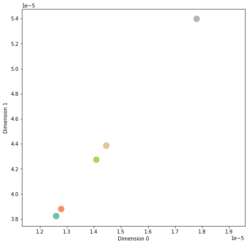
2. Node classification on Cora Dataset
Prelims
import math
import numpy as np
import scipy.sparse as sp
import torch
import torch.nn as nn
import torch.nn.functional as F
from torch.nn.parameter import Parameter
from torch.nn.modules.module import Module
import torch.optim as optim
import time
Cora Dataset
Dataset link : https://relational.fit.cvut.cz/dataset/CORA
The Cora dataset consists of 2708 scientific publications classified into one of seven classes. The citation network consists of 5429 links. Each publication in the dataset is described by a 0/1-valued word vector indicating the absence/presence of the corresponding word from the dictionary. The dictionary consists of 1433 unique words.
!wget https://www.dropbox.com/s/fl9mvrio3hah4on/cora.content
!wget https://www.dropbox.com/s/l829sldp7xqrt0h/cora.cites
--2023-03-29 04:33:24-- https://www.dropbox.com/s/fl9mvrio3hah4on/cora.content
Resolving www.dropbox.com (www.dropbox.com)... 162.125.5.18, 2620:100:601d:18::a27d:512
Connecting to www.dropbox.com (www.dropbox.com)|162.125.5.18|:443... connected.
HTTP request sent, awaiting response... 302 Found
Location: /s/raw/fl9mvrio3hah4on/cora.content [following]
--2023-03-29 04:33:24-- https://www.dropbox.com/s/raw/fl9mvrio3hah4on/cora.content
Reusing existing connection to www.dropbox.com:443.
HTTP request sent, awaiting response... 302 Found
Location: https://ucc707d5f870402527cddc2e884d.dl.dropboxusercontent.com/cd/0/inline/B5I2a5oebS3gQKwwE1pf10_TTs_zsaTq85HHdsETKp31dwf53tn-nmhwTTOi3bz2SXgHrW3f3rODqNgQKdDkdpqloOM1EVudixBr1kutr51CQOpYKcnAhKbjkeie3Y2LCFBEXuRuOqOZBPtCQnRQHPJ9t4Ki3pvXDxNVCej0syBteg/file# [following]
--2023-03-29 04:33:25-- https://ucc707d5f870402527cddc2e884d.dl.dropboxusercontent.com/cd/0/inline/B5I2a5oebS3gQKwwE1pf10_TTs_zsaTq85HHdsETKp31dwf53tn-nmhwTTOi3bz2SXgHrW3f3rODqNgQKdDkdpqloOM1EVudixBr1kutr51CQOpYKcnAhKbjkeie3Y2LCFBEXuRuOqOZBPtCQnRQHPJ9t4Ki3pvXDxNVCej0syBteg/file
Resolving ucc707d5f870402527cddc2e884d.dl.dropboxusercontent.com (ucc707d5f870402527cddc2e884d.dl.dropboxusercontent.com)... 162.125.5.15, 2620:100:601d:15::a27d:50f
Connecting to ucc707d5f870402527cddc2e884d.dl.dropboxusercontent.com (ucc707d5f870402527cddc2e884d.dl.dropboxusercontent.com)|162.125.5.15|:443... connected.
HTTP request sent, awaiting response... 200 OK
Length: 7823427 (7.5M) [text/plain]
Saving to: ‘cora.content’
cora.content 100%[===================>] 7.46M 26.6MB/s in 0.3s
2023-03-29 04:33:25 (26.6 MB/s) - ‘cora.content’ saved [7823427/7823427]
--2023-03-29 04:33:25-- https://www.dropbox.com/s/l829sldp7xqrt0h/cora.cites
Resolving www.dropbox.com (www.dropbox.com)... 162.125.5.18, 2620:100:601d:18::a27d:512
Connecting to www.dropbox.com (www.dropbox.com)|162.125.5.18|:443... connected.
HTTP request sent, awaiting response... 302 Found
Location: /s/raw/l829sldp7xqrt0h/cora.cites [following]
--2023-03-29 04:33:26-- https://www.dropbox.com/s/raw/l829sldp7xqrt0h/cora.cites
Reusing existing connection to www.dropbox.com:443.
HTTP request sent, awaiting response... 302 Found
Location: https://uc7299ce09e72c10e019548e02ea.dl.dropboxusercontent.com/cd/0/inline/B5L_KRMUSNoZuJrAFF1ohIQJIfIMY4rtPkkHmxd8Nf3rYNFHP8mcBY5jOht_FehBKOg61tPXEvZzP9A2rGDqOrTh2rVTzvzfr9SKKZ1-DNMhIZXtXY_RmLm9PvhsT3G83r4F-R0jNSYB1j-dgen8-aSeHX28dSkuaKr4UQtvVNm1qQ/file# [following]
--2023-03-29 04:33:26-- https://uc7299ce09e72c10e019548e02ea.dl.dropboxusercontent.com/cd/0/inline/B5L_KRMUSNoZuJrAFF1ohIQJIfIMY4rtPkkHmxd8Nf3rYNFHP8mcBY5jOht_FehBKOg61tPXEvZzP9A2rGDqOrTh2rVTzvzfr9SKKZ1-DNMhIZXtXY_RmLm9PvhsT3G83r4F-R0jNSYB1j-dgen8-aSeHX28dSkuaKr4UQtvVNm1qQ/file
Resolving uc7299ce09e72c10e019548e02ea.dl.dropboxusercontent.com (uc7299ce09e72c10e019548e02ea.dl.dropboxusercontent.com)... 162.125.5.15, 2620:100:601d:15::a27d:50f
Connecting to uc7299ce09e72c10e019548e02ea.dl.dropboxusercontent.com (uc7299ce09e72c10e019548e02ea.dl.dropboxusercontent.com)|162.125.5.15|:443... connected.
HTTP request sent, awaiting response... 200 OK
Length: 69928 (68K) [text/plain]
Saving to: ‘cora.cites’
cora.cites 100%[===================>] 68.29K --.-KB/s in 0.03s
2023-03-29 04:33:26 (1.94 MB/s) - ‘cora.cites’ saved [69928/69928]import pandas as pd
import os
edgelist = pd.read_csv(os.path.join("./", "cora.cites"), sep='\t', header=None, names=["target", "source"]) # it has graph
edgelist["label"] = "cites"
edgelist.sample(frac=1).head(5) # <ID of cited paper node> <ID of citing paper node>, by doing this, you can see the edge information| target | source | label | |
|---|---|---|---|
| 4294 | 152731 | 1109392 | cites |
| 2625 | 28385 | 118558 | cites |
| 4255 | 144408 | 219446 | cites |
| 3696 | 78555 | 78557 | cites |
| 437 | 1365 | 188318 | cites |
<svg xmlns="http://www.w3.org/2000/svg" height="24px"viewBox="0 0 24 24"
width="24px">
  <script>
    const buttonEl =
      document.querySelector('#df-61e82418-b31c-44c8-8f8f-4b3517da82c7 button.colab-df-convert');
    buttonEl.style.display =
      google.colab.kernel.accessAllowed ? 'block' : 'none';

    async function convertToInteractive(key) {
      const element = document.querySelector('#df-61e82418-b31c-44c8-8f8f-4b3517da82c7');
      const dataTable =
        await google.colab.kernel.invokeFunction('convertToInteractive',
                                                 [key], {});
      if (!dataTable) return;

      const docLinkHtml = 'Like what you see? Visit the ' +
        '<a target="_blank" href=https://colab.research.google.com/notebooks/data_table.ipynb>data table notebook</a>'
        + ' to learn more about interactive tables.';
      element.innerHTML = '';
      dataTable['output_type'] = 'display_data';
      await google.colab.output.renderOutput(dataTable, element);
      const docLink = document.createElement('div');
      docLink.innerHTML = docLinkHtml;
      element.appendChild(docLink);
    }
  </script>
</div>
Gnx = nx.from_pandas_edgelist(edgelist, edge_attr="label")
nx.set_node_attributes(Gnx, "paper", "label")
print(Gnx.nodes) # from edgelist, by using from_pandas_edgelist() function, we can extract node list from edgelist
Gnx.nodes[12210] ## by type this, we can see the node feature[1033, 35, 103482, 103515, 1050679, 1103960, 1103985, 1109199, 1112911, 1113438, 1113831, 1114331, 1117476, 1119505, 1119708, 1120431, 1123756, 1125386, 1127430, 1127913, 1128204, 1128227, 1128314, 1128453, 1128945, 1128959, 1128985, 1129018, 1129027, 1129573, 1129683, 1129778, 1130847, 1130856, 1131116, 1131360, 1131557, 1131752, 1133196, 1133338, 1136814, 1137466, 1152421, 1152508, 1153065, 1153280, 1153577, 1153853, 1153943, 1154176, 1154459, 116552, 12576, 128540, 132806, 135130, 141342, 141347, 148170, 15670, 1688, 175291, 178727, 18582, 190697, 190706, 1956, 197054, 198443, 198653, 206371, 210871, 229635, 231249, 248425, 249421, 254923, 259701, 259702, 263279, 263498, 265203, 273152, 27510, 28290, 286500, 287787, 28851, 289779, 289780, 289781, 307015, 335733, 33904, 33907, 35061, 38205, 387795, 415693, 41714, 427606, 44368, 45599, 46079, 46431, 486840, 48766, 503883, 503893, 513189, 54129, 54131, 56119, 561238, 568857, 573964, 573978, 574009, 574264, 574462, 575077, 575292, 575331, 576725, 576795, 577227, 578780, 579008, 592973, 593091, 593105, 593240, 593260, 593813, 594047, 594543, 594649, 594900, 608326, 634902, 634904, 634938, 634975, 640617, 646809, 646837, 647408, 647447, 66556, 66563, 66805, 69284, 69296, 694759, 735303, 78511, 787016, 801170, 81722, 82098, 84021, 85352, 86359, 8865, 887, 97645, 98698, 1109017, 40, 1114442, 1103315, 114, 1105394, 1106112, 1106172, 1106406, 1107455, 1111052, 1114125, 1117942, 1118245, 1118332, 1120170, 1126029, 124064, 128, 130, 136665, 191404, 193742, 23258, 28227, 28287, 28350, 28387, 28471, 28485, 341188, 38480, 39403, 434, 55968, 58540, 6155, 6170, 6196, 6220, 64484, 7432, 755217, 8213, 91975, 976334, 1109581, 117, 149669, 17476, 189708, 206259, 28202, 28278, 32872, 33013, 6214, 75674, 20526, 13960, 345340, 1118092, 288, 36167, 1135125, 424, 218666, 47684, 267003, 58454, 463, 1102364, 504, 1112650, 506, 89416, 1106546, 10796, 1105033, 1111304, 1113614, 114308, 134128, 161221, 170798, 19045, 20972, 28456, 299195, 299197, 334153, 35490, 595056, 6151, 6213, 6215, 64519, 87363, 1103979, 906, 1105344, 1114352, 1136397, 1140040, 34355, 910, 1104379, 1105530, 1108834, 1110520, 1114118, 1116569, 1118848, 1120858, 1122460, 1126044, 1129111, 1135137, 1152194, 12439, 12946, 131042, 13136, 160705, 227286, 242637, 31043, 340075, 340078, 35905, 42847, 436796, 48550, 5462, 576257, 58552, 5869, 636511, 67292, 675649, 684372, 94953, 1107010, 936, 1111899, 129558, 207395, 3084, 3828, 38845, 20180, 940, 28265, 941, 1152896, 943, 91852, 1034, 1026, 1102550, 1105231, 1129798, 1153945, 1107062, 1035, 1110515, 1154525, 1213, 409725, 8766, 102938, 1237, 1102400, 143676, 1246, 1104007, 42207, 57764, 6125, 1102625, 1272, 1108167, 1120962, 112378, 1123867, 1128256, 1129208, 1135358, 157805, 18615, 192734, 20593, 27230, 284414, 30895, 30901, 444240, 520471, 52835, 552469, 560936, 591016, 636098, 65653, 6917, 6923, 85452, 85688, 93923, 97892, 1031453, 1365, 1102407, 1105062, 1106287, 1108050, 1110494, 1110998, 1113995, 1114153, 1114388, 1114605, 1116347, 1116594, 1117653, 1119140, 1120211, 1120866, 1128839, 1129443, 1130600, 1131647, 1131745, 1131748, 1132922, 1132968, 1135368, 1136422, 1136442, 1152143, 1152821, 1154169, 120084, 139865, 157401, 171225, 184918, 188318, 188471, 22835, 23448, 23502, 23507, 237521, 26850, 330148, 340299, 39904, 49482, 562123, 628500, 648232, 649731, 69392, 7276, 7297, 77758, 782486, 83826, 85299, 853150, 90888, 93555, 948299, 948846, 949318, 949511, 950052, 950305, 1102567, 1481, 1106052, 1108267, 1111614, 1113934, 1114864, 1117184, 1119295, 1120563, 1153891, 200480, 399173, 4878, 521207, 521269, 1134022, 152483, 1694, 39474, 647413, 1115291, 1717, 1116336, 1135108, 50381, 733167, 35797, 1786, 1114502, 1817, 1108389, 1919, 129042, 1949, 3101, 3095, 1951, 1107215, 1952, 1153166, 1953, 1153724, 1153728, 110163, 1955, 1110390, 101143, 1118302, 1153101, 1153150, 263486, 83449, 1959, 3097, 310530, 38839, 73327, 82664, 1102442, 1997, 1108551, 1109439, 1109542, 129897, 154982, 3233, 49811, 7032, 1999, 1123068, 1131471, 39126, 6771, 10186, 2354, 1107140, 1113852, 1130539, 154134, 40151, 74749, 1000012, 2440, 1061127, 1106388, 1107095, 1110426, 1114512, 1117786, 1120650, 1127619, 1153254, 136766, 136768, 151430, 212777, 23546, 49843, 49844, 49847, 582343, 591017, 63931, 72908, 102406, 2653, 107177, 1104055, 1116268, 1116842, 1118764, 1119751, 1152075, 167656, 197783, 28641, 321861, 350362, 4660, 59045, 65650, 1104851, 2654, 1106630, 1107861, 1110438, 1121867, 1123926, 211906, 27250, 463825, 52784, 1115375, 2658, 1130676, 1130808, 1131607, 1132948, 1135899, 1140230, 230884, 236759, 282700, 395540, 578347, 696342, 696345, 696346, 751408, 99023, 1119671, 2663, 1105574, 2665, 1113035, 1122704, 1132486, 205192, 237489, 43639, 578306, 578309, 578337, 582139, 630817, 631052, 763009, 1108169, 2695, 1120197, 2698, 342802, 2696, 1114192, 1118083, 1123239, 1133004, 256106, 469504, 5348, 99025, 1120777, 2702, 12330, 395553, 72056, 1107171, 255233, 33303, 15889, 3085, 221302, 30973, 395725, 5062, 110162, 218682, 1106236, 129045, 110164, 70441, 103529, 3112, 1152564, 470511, 77826, 77829, 1110000, 3187, 129896, 280876, 5086, 105865, 3191, 1106789, 1127530, 1131267, 137873, 162664, 308920, 310742, 3192, 423463, 561364, 642827, 3217, 167670, 238099, 86840, 1106492, 3218, 1119987, 1120169, 1152290, 1153264, 187354, 277263, 35070, 417017, 6639, 66782, 6767, 6941, 1115677, 3220, 1125992, 1128430, 1130634, 1131728, 1132706, 120039, 145215, 346243, 36620, 39124, 40922, 429805, 654177, 69397, 8832, 1103737, 3222, 1114222, 1131137, 1132157, 964248, 3223, 100197, 3229, 1105718, 1106568, 1108209, 1109392, 1112767, 1125082, 1125895, 1126037, 1128868, 1130915, 1130927, 1130931, 1132418, 1140289, 1152277, 1152673, 1154251, 118559, 133550, 16461, 189577, 25181, 25184, 27174, 27631, 31769, 33412, 35343, 35863, 35922, 390922, 396412, 444191, 447250, 52515, 62347, 641976, 654326, 7022, 72101, 82087, 919885, 92065, 96335, 104840, 3231, 1102761, 1106330, 1106370, 1107067, 1113926, 1115471, 1128536, 1153169, 180399, 20850, 259126, 3237, 328370, 49660, 6334, 63477, 63486, 66594, 68463, 8699, 8821, 3232, 20942, 521251, 1125467, 192850, 272720, 509379, 976284, 3235, 3236, 601561, 1110531, 3240, 39130, 1103610, 3243, 1110947, 1113739, 307336, 31932, 368431, 854434, 5075, 3932, 1105428, 4274, 1114664, 1119078, 105899, 4329, 1110768, 28254, 395547, 46468, 510718, 1103676, 4330, 1104449, 11093, 1112929, 1132459, 1132461, 1136393, 1152917, 118436, 119956, 120013, 151708, 168410, 32688, 37884, 390889, 428610, 684986, 69418, 753265, 949217, 1104300, 4335, 1121254, 1136310, 1140547, 116790, 239800, 32698, 62274, 62417, 755082, 95718, 1102548, 4553, 4584, 1120020, 1130567, 13885, 13917, 293285, 6184, 6210, 628815, 164, 4637, 1105887, 4649, 1127851, 135765, 135766, 411092, 449841, 8703, 429781, 5038, 102884, 4804, 1108175, 1112574, 1153262, 12182, 12210, 157761, 25805, 45189, 68505, 77515, 989397, 7867, 4983, 5055, 28026, 5064, 5069, 1121176, 1129106, 272345, 385067, 109323, 1105698, 137849, 354004, 440815, 79809, 1152714, 5194, 133563, 133566, 140569, 139547, 75695, 911198, 5454, 1128425, 1130680, 1022969, 5600, 1117833, 5959, 152226, 545647, 582511, 5966, 1107572, 12211, 27612, 385251, 6130, 1154123, 1154124, 671269, 675847, 1106547, 1107355, 1385, 6152, 1106966, 6163, 20534, 96847, 6169, 1114629, 170338, 7419, 10981, 1120731, 13686, 399339, 1153056, 81350, 1108329, 6209, 118259, 118260, 181782, 212930, 8875, 95579, 1105764, 1109957, 1111230, 1113182, 1113459, 1117760, 1122425, 1123553, 1128267, 1129096, 1129243, 13193, 153598, 17208, 195361, 218410, 23774, 241133, 293271, 353541, 6224, 628667, 628668, 672064, 1115886, 1152740, 28447, 6378, 93320, 95589, 6216, 230300, 10793, 6238, 1123991, 1130356, 84459, 6311, 235776, 1108656, 6318, 1121057, 20833, 1152307, 1152448, 1152975, 1153703, 6343, 141868, 359067, 521252, 1112665, 6344, 1106103, 6346, 1112075, 28473, 1103162, 6385, 682666, 892139, 1102646, 6539, 116084, 178209, 568045, 1130637, 6741, 1153160, 348437, 49895, 51909, 83725, 9708, 1120444, 6925, 1111240, 6775, 350319, 6782, 100961, 6784, 1116629, 60170, 6786, 714975, 1117348, 6814, 1125469, 158172, 293974, 300071, 315266, 390896, 445938, 1105531, 6818, 50336, 50337, 1123188, 6898, 124224, 12631, 431206, 6910, 78994, 1117219, 1132083, 1152150, 1154103, 169279, 263553, 662416, 1105011, 6913, 1131230, 703953, 1153811, 1155073, 20857, 308003, 1114526, 1118658, 372862, 57922, 57948, 6935, 101660, 1115670, 1116922, 6939, 323128, 52847, 1120880, 7041, 1135082, 7047, 14549, 54844, 1136446, 7272, 763181, 7296, 763010, 1107312, 1153287, 7430, 95586, 1121603, 7532, 1153097, 141171, 314459, 7537, 80515, 1113534, 1131348, 409255, 1138027, 315789, 105057, 8079, 1108728, 8224, 1111788, 1128531, 1132815, 11342, 1153148, 1153866, 133615, 22431, 22563, 23738, 55403, 601567, 62389, 97377, 1120059, 8581, 75691, 8591, 137956, 167205, 709113, 1132809, 8594, 180187, 232605, 58268, 8617, 12359, 36145, 8619, 1102751, 8687, 38000, 8696, 101145, 173884, 27535, 308232, 502574, 51866, 59244, 89335, 1129570, 395075, 608292, 785678, 1104647, 8872, 1125092, 1152761, 1153860, 1120643, 8874, 1153816, 1152676, 8961, 1133390, 102879, 9513, 9515, 1102794, 9559, 252725, 1130780, 9581, 633585, 1120138, 9586, 33818, 1153003, 9716, 28674, 10169, 114189, 158614, 17798, 211875, 39131, 711598, 10174, 10177, 12197, 12198, 124734, 15429, 249858, 27606, 67415, 68495, 10183, 10430, 1114336, 1120713, 259772, 47570, 54550, 1103394, 10435, 208345, 22566, 41417, 1102850, 10531, 1107567, 1129442, 194617, 31336, 31349, 31353, 43698, 686532, 180373, 31097, 46536, 6217, 10798, 1154500, 18619, 20193, 252715, 1102873, 39199, 1129835, 11148, 1131719, 193354, 25413, 11339, 11326, 1127657, 11335, 11325, 217139, 11337, 211432, 44017, 45061, 1126350, 12155, 12199, 12158, 148399, 12165, 1112099, 1119471, 12169, 1059953, 1106418, 1117249, 1153183, 155736, 219239, 28632, 28640, 309476, 94713, 27199, 12194, 1107319, 12195, 1131611, 1132285, 38722, 51180, 111866, 95225, 12247, 101263, 12238, 107569, 1152490, 1153861, 156977, 213279, 400356, 12337, 16451, 16470, 16474, 12347, 101811, 12350, 152227, 20601, 20602, 1131634, 1071981, 1104999, 1105221, 1107674, 127033, 416455, 56112, 56709, 574710, 575795, 62718, 63832, 12638, 119761, 899119, 13024, 13195, 1105148, 13205, 13208, 131318, 13212, 214472, 358884, 411005, 13213, 13269, 13654, 13652, 13656, 83746, 1115959, 119686, 987188, 13658, 294239, 13717, 37998, 13966, 1126050, 13972, 34979, 13982, 14062, 1152358, 646836, 97390, 98693, 1103016, 14083, 14090, 643069, 1103031, 14428, 1103969, 14429, 14431, 34082, 73119, 1119216, 14430, 1103038, 14529, 239829, 14531, 1105932, 1152308, 56167, 592830, 60682, 14545, 14807, 264347, 25702, 15076, 708945, 175576, 210309, 217115, 35854, 41666, 89547, 15431, 12558, 1110024, 1118388, 15892, 175909, 1116146, 158098, 15984, 15987, 523394, 653441, 714289, 16008, 1131165, 189571, 189572, 152219, 16437, 430329, 51831, 1105603, 1129621, 1104787, 16471, 1114992, 273949, 1123087, 16476, 105856, 16485, 1109891, 1120049, 1131167, 16819, 1131236, 1131274, 1131312, 126793, 643003, 643221, 644093, 644334, 646195, 646286, 1152259, 16843, 1152991, 17201, 1126012, 184157, 95435, 1152633, 17242, 17363, 17477, 17488, 1107136, 17811, 245955, 17821, 18251, 18313, 86923, 18532, 1106854, 18536, 424540, 1153091, 28964, 18770, 531348, 531351, 18773, 88356, 73146, 18774, 103537, 18777, 1112686, 173863, 66794, 79817, 18781, 18785, 1106401, 18811, 20920, 18812, 510715, 18815, 18832, 18833, 18834, 1152944, 593210, 593328, 593329, 19231, 1153736, 12960, 30934, 686061, 19621, 1128846, 1131464, 123825, 240791, 628888, 649730, 649739, 66990, 853116, 948147, 19697, 40124, 38829, 20178, 64271, 91853, 20179, 95188, 1108597, 1114777, 1116397, 1116839, 1119180, 112813, 1130653, 1130657, 1138091, 1152244, 1153877, 1153879, 1153889, 144330, 566488, 566653, 566664, 20528, 70442, 1106849, 20584, 1118823, 20592, 389715, 1118209, 1121537, 20821, 1127863, 1115701, 20923, 1116530, 20924, 289885, 294030, 1116181, 1103383, 22229, 1107418, 1128369, 144701, 22241, 243483, 459216, 595193, 22386, 1128407, 38846, 107251, 107252, 1121459, 22564, 36140, 63915, 94229, 1110563, 22876, 22869, 22874, 22875, 22883, 1107367, 22886, 23070, 23069, 74700, 1116044, 134307, 134316, 74698, 87915, 1105433, 23116, 1111978, 152731, 217852, 101662, 1153064, 189574, 27249, 84020, 1111265, 24043, 928873, 1103499, 24476, 1153024, 24530, 24966, 1106671, 1123576, 1131149, 1154042, 124828, 145134, 145176, 197452, 202639, 27627, 63549, 65212, 671293, 95719, 1104258, 24974, 1112723, 34315, 40125, 285675, 385572, 1153897, 147870, 1104769, 25772, 1122580, 1126503, 641956, 25791, 45212, 25794, 1110028, 1121063, 248119, 27203, 23545, 27241, 27243, 27246, 1128990, 27514, 27530, 1128542, 27531, 592826, 1112026, 34961, 27543, 27623, 1104182, 27632, 686015, 686030, 116021, 27895, 325497, 28230, 28249, 1152436, 28267, 308529, 567005, 108047, 28336, 28359, 28385, 118558, 28389, 28412, 194645, 28487, 28489, 1152910, 28491, 1139928, 28504, 131315, 365294, 28542, 32260, 28649, 155738, 578669, 595157, 28957, 159897, 1125402, 1125944, 1112426, 29492, 1122574, 131117, 144408, 29708, 400473, 29723, 155277, 29738, 30817, 144679, 31055, 31083, 48066, 1105672, 31105, 1063773, 1124844, 1129608, 1135746, 1152162, 1152272, 1152904, 286562, 31927, 686559, 31479, 39165, 31483, 118682, 31489, 40583, 40605, 632796, 632874, 632935, 633721, 67245, 67246, 358894, 31863, 91581, 1129572, 32083, 1153933, 200630, 346292, 45605, 688361, 32276, 174418, 636500, 84695, 33231, 1132887, 33301, 1110256, 33325, 124296, 34708, 78549, 78552, 78557, 1119004, 33823, 33895, 1110546, 1106771, 34257, 1111186, 1114398, 1115456, 1116974, 1122642, 192870, 34263, 34266, 368605, 87482, 90655, 503871, 682815, 168958, 35335, 59772, 1104031, 1116410, 108962, 35778, 108983, 519318, 1128974, 399370, 60169, 627024, 35852, 41732, 134060, 1105116, 194223, 390894, 66982, 36131, 77438, 350373, 46500, 36162, 189620, 36802, 189856, 37888, 589923, 590022, 37483, 37541, 260979, 37879, 1128997, 1129610, 1153942, 117316, 592975, 592986, 593060, 606647, 61069, 1131270, 38537, 1131277, 137868, 153063, 642847, 1104191, 38771, 1110579, 39127, 1128881, 1128927, 1128935, 116081, 116087, 195150, 46476, 75972, 39210, 66986, 1123689, 39890, 1154229, 1154232, 1154233, 242663, 51045, 521855, 559804, 714256, 118079, 40131, 40135, 1104261, 884094, 40886, 41216, 1113551, 128383, 943087, 144212, 182094, 44455, 42156, 1118120, 1152179, 42209, 42221, 42848, 1116835, 1131195, 43165, 1135894, 43186, 206524, 48075, 1104435, 44121, 227178, 44514, 253971, 606479, 1131266, 45052, 1130929, 45188, 1105450, 1132385, 1104495, 45533, 45603, 1131639, 975567, 1152569, 46452, 46470, 46491, 137380, 46547, 51834, 1153275, 46501, 46887, 1153106, 1125393, 47682, 47683, 1124837, 47839, 48555, 48764, 48768, 48781, 1134865, 397488, 423816, 1112369, 217984, 49753, 49720, 683355, 123556, 50354, 289088, 1104749, 50807, 50838, 73972, 50980, 1134320, 51049, 51052, 51879, 51934, 1104809, 52000, 52007, 52003, 1112194, 300806, 446271, 53942, 1128291, 1128319, 1136791, 117315, 578645, 578646, 578649, 593022, 1128982, 141324, 459213, 459214, 593859, 593942, 59715, 54132, 593921, 594387, 62634, 1104946, 55770, 55801, 56115, 1119178, 239810, 56708, 57119, 1132731, 711527, 1154524, 57773, 235670, 57932, 1114239, 58436, 87417, 58453, 1113828, 248395, 58758, 1128208, 576973, 59626, 96845, 59798, 60159, 61073, 61312, 1106764, 61417, 94416, 1131565, 62329, 195792, 251756, 593155, 650834, 62333, 1107325, 1107558, 294145, 62607, 62676, 312409, 83461, 1105360, 63812, 63835, 64319, 1125909, 65057, 519353, 1110209, 65074, 1117920, 142268, 714748, 1112319, 1123530, 66564, 362926, 66596, 1135750, 66751, 1138043, 573535, 693143, 695284, 1105505, 1153031, 509315, 82090, 66809, 1117501, 171954, 1127558, 67584, 1127566, 562067, 67633, 68115, 68224, 231198, 69198, 70281, 70444, 70520, 70970, 593068, 71336, 71736, 71904, 1135122, 1118347, 72406, 899085, 72805, 954315, 73162, 1134348, 189774, 714260, 714879, 1105810, 73323, 73712, 74427, 1120252, 74821, 1131150, 1105877, 74920, 74921, 74937, 1107041, 74975, 75121, 103430, 75318, 1121569, 75693, 75694, 75969, 1128856, 75983, 1115790, 77108, 77112, 106590, 1129994, 1129907, 613409, 78508, 575402, 78555, 662279, 662572, 1121659, 1131466, 358866, 80491, 80656, 81714, 82666, 82920, 1125492, 1128198, 1129367, 576691, 83847, 1130678, 1106298, 1133047, 509233, 85324, 628751, 577086, 85449, 86258, 1133469, 1114184, 1153786, 89308, 103528, 137130, 1116328, 1152379, 237376, 90470, 91038, 92589, 93273, 93318, 1152958, 143801, 284023, 284025, 93755, 1111733, 94639, 94641, 116553, 95198, 95588, 95594, 95597, 95642, 990075, 594025, 96851, 100935, 99030, 193931, 100701, 596075, 101261, 102061, 102939, 1154074, 1113742, 246618, 103531, 656048, 126912, 103543, 126927, 289085, 193932, 1095507, 1107385, 1153899, 578898, 108963, 310653, 108974, 1133417, 683404, 110041, 111676, 1119623, 111770, 112099, 112787, 1125258, 114966, 1107728, 115188, 1107808, 116512, 116528, 116545, 1115166, 117328, 118424, 118435, 1121739, 1109566, 118873, 119712, 1140543, 1109873, 120817, 1152394, 121792, 141160, 1154276, 1119742, 124952, 1126011, 189721, 1108258, 126867, 126868, 126909, 126920, 645897, 126926, 1114364, 127940, 243274, 128202, 128203, 1108363, 1121313, 907845, 129287, 131122, 131317, 132821, 133553, 133567, 1108570, 133628, 481073, 134199, 164885, 447224, 134219, 134314, 134315, 134320, 135464, 1135589, 135798, 136767, 137359, 1118286, 137790, 1131300, 1154068, 139738, 1108841, 140005, 1131345, 917493, 503877, 608191, 141596, 143323, 143476, 1131549, 219446, 1128975, 1136342, 595063, 294126, 145315, 649944, 145384, 1109185, 1132434, 1109208, 148341, 1123215, 149139, 1120786, 987197, 583318, 1131223, 561568, 561581, 561593, 561595, 561610, 561613, 645084, 1112106, 154023, 1133846, 154047, 1130934, 1133028, 397590, 155158, 156794, 1118017, 1127812, 158812, 1152711, 159084, 159085, 241821, 1128853, 160732, 1153922, 1109830, 162075, 162080, 737204, 1135345, 739707, 163235, 166420, 166825, 166989, 168332, 169280, 656231, 1138755, 820662, 174425, 175256, 175548, 689152, 753070, 177115, 177993, 177998, 178718, 179180, 179702, 1152859, 179706, 1110628, 180301, 1120084, 182093, 1131550, 650814, 1110950, 187260, 1153014, 189566, 189623, 189655, 1129518, 1134346, 190698, 191216, 191222, 193347, 612306, 193352, 193918, 194609, 1154520, 126128, 215912, 563613, 248823, 377303, 198866, 199571, 643734, 202520, 202522, 643597, 203646, 205196, 1130568, 1130586, 628764, 628766, 815096, 950986, 1128151, 1129629, 210872, 1112071, 212097, 212107, 213246, 1117618, 216877, 216878, 1152663, 1112417, 219218, 567018, 219976, 220420, 226698, 1122304, 1128946, 228992, 228990, 230879, 1133428, 696343, 851968, 1153195, 232606, 1113084, 232860, 12275, 233106, 630890, 235678, 235679, 689439, 235683, 238401, 240321, 1113541, 245288, 1121398, 248431, 250566, 253762, 255628, 258259, 260121, 261040, 262108, 262121, 262178, 1138968, 263069, 263482, 264556, 335042, 267824, 270456, 1114838, 270600, 278394, 278403, 1152959, 285687, 286513, 288107, 1153784, 289945, 578845, 292277, 1133010, 1152858, 302545, 1131198, 643199, 307656, 270085, 1139195, 318071, 318187, 1117049, 321004, 1117089, 325314, 330208, 337766, 348305, 1118546, 358887, 360028, 1119211, 367312, 746058, 400455, 368657, 370366, 375605, 375825, 1119654, 376704, 379288, 60560, 380341, 1120019, 384428, 390693, 684972, 1135115, 1154173, 408885, 416867, 416964, 421481, 1105622, 430574, 1132416, 430711, 671052, 645571, 446610, 1123093, 1123493, 458439, 459206, 466170, 1128977, 467383, 1131374, 1154076, 577331, 646913, 1125597, 1125906, 1125953, 521183, 1125993, 1132864, 522338, 683360, 523010, 523574, 1126315, 529165, 561582, 646440, 561611, 1127541, 561674, 1127551, 561789, 561809, 562940, 1127810, 573553, 1138970, 593544, 608190, 1131734, 576362, 1128201, 578365, 1153900, 578650, 1128943, 1128978, 593559, 593560, 579108, 1128437, 582349, 592993, 592996, 593248, 1129015, 593104, 593201, 593209, 1153896, 594011, 594039, 1129021, 594119, 1129040, 594483, 594511, 601462, 1129368, 1129369, 1129494, 604073, 1153946, 610529, 616336, 1130069, 617378, 1130080, 617575, 1130243, 621555, 1130454, 626530, 1154012, 626531, 626574, 626999, 628459, 628458, 631015, 633031, 633030, 633081, 672070, 672071, 1131163, 642593, 1131164, 642621, 1131258, 642641, 642681, 644441, 1131172, 642798, 644470, 1131180, 642894, 1131301, 1131335, 643239, 643485, 645046, 645870, 646334, 646357, 1131184, 642920, 642930, 1131189, 1131192, 1131257, 1131305, 1131334, 644448, 644577, 643695, 643777, 643735, 645016, 644361, 644363, 644427, 1131314, 644494, 644843, 1154071, 645088, 645452, 646289, 1131330, 646412, 1131359, 646900, 647315, 1131421, 648106, 648112, 1131420, 648121, 1131414, 648369, 650807, 1133930, 653628, 1131741, 654339, 1131754, 654519, 1131828, 1132073, 662250, 1132406, 1132443, 1132505, 675756, 1132857, 682508, 683294, 684531, 687401, 1133008, 688824, 688849, 1134031, 1134056, 709518, 1134197, 711994, 714208, 1154230, 733534, 733576, 734406, 735311, 1135455, 738941, 739280, 739816, 1140548, 1135955, 752684, 1136631, 753047, 1136634, 753264, 767763, 1136040, 754594, 1136110, 756061, 1136447, 762980, 1136449, 1137140, 779960, 1138619, 814836, 815073, 820661, 817774, 1139009, 824245, 1140231, 853114, 853155, 853115, 853118]
{'label': 'paper'}feature_names = ["word_{}".format(ii) for ii in range(1433)]
column_names = feature_names + ["subject"]
node_data = pd.read_csv(os.path.join("/content/", "cora.content"), sep='\t', header=None, names=column_names)
node_data.head(5) # <paper node id> <word_attributes>+ <node label>| word_0 | word_1 | word_2 | word_3 | word_4 | word_5 | word_6 | word_7 | word_8 | word_9 | ... | word_1424 | word_1425 | word_1426 | word_1427 | word_1428 | word_1429 | word_1430 | word_1431 | word_1432 | subject | |
|---|---|---|---|---|---|---|---|---|---|---|---|---|---|---|---|---|---|---|---|---|---|
| 31336 | 0 | 0 | 0 | 0 | 0 | 0 | 0 | 0 | 0 | 0 | ... | 0 | 0 | 1 | 0 | 0 | 0 | 0 | 0 | 0 | Neural_Networks |
| 1061127 | 0 | 0 | 0 | 0 | 0 | 0 | 0 | 0 | 0 | 0 | ... | 0 | 1 | 0 | 0 | 0 | 0 | 0 | 0 | 0 | Rule_Learning |
| 1106406 | 0 | 0 | 0 | 0 | 0 | 0 | 0 | 0 | 0 | 0 | ... | 0 | 0 | 0 | 0 | 0 | 0 | 0 | 0 | 0 | Reinforcement_Learning |
| 13195 | 0 | 0 | 0 | 0 | 0 | 0 | 0 | 0 | 0 | 0 | ... | 0 | 0 | 0 | 0 | 0 | 0 | 0 | 0 | 0 | Reinforcement_Learning |
| 37879 | 0 | 0 | 0 | 0 | 0 | 0 | 0 | 0 | 0 | 0 | ... | 0 | 0 | 0 | 0 | 0 | 0 | 0 | 0 | 0 | Probabilistic_Methods |
5 rows × 1434 columns
<svg xmlns="http://www.w3.org/2000/svg" height="24px"viewBox="0 0 24 24"
width="24px">
  <script>
    const buttonEl =
      document.querySelector('#df-ce86d877-4c6c-48e3-b484-2f62f22a693d button.colab-df-convert');
    buttonEl.style.display =
      google.colab.kernel.accessAllowed ? 'block' : 'none';

    async function convertToInteractive(key) {
      const element = document.querySelector('#df-ce86d877-4c6c-48e3-b484-2f62f22a693d');
      const dataTable =
        await google.colab.kernel.invokeFunction('convertToInteractive',
                                                 [key], {});
      if (!dataTable) return;

      const docLinkHtml = 'Like what you see? Visit the ' +
        '<a target="_blank" href=https://colab.research.google.com/notebooks/data_table.ipynb>data table notebook</a>'
        + ' to learn more about interactive tables.';
      element.innerHTML = '';
      dataTable['output_type'] = 'display_data';
      await google.colab.output.renderOutput(dataTable, element);
      const docLink = document.createElement('div');
      docLink.innerHTML = docLinkHtml;
      element.appendChild(docLink);
    }
  </script>
</div>set(node_data["subject"]) # node class type{'Case_Based',
'Genetic_Algorithms',
'Neural_Networks',
'Probabilistic_Methods',
'Reinforcement_Learning',
'Rule_Learning',
'Theory'}In the class, we will predict the subject of a paper (node) on the basis of the surrounding node data and the structure of the graph.
Hyperparameter
EPOCH = 200
SEED = 42
NUM_HIDDEN = 16
dropout_rate = 0.5
learning_rate = 0.01
weight_decay = 5e-4
Preprocess and Make Dataset
def encode_onehot(labels): # we will make all class(subject) to one-hot vector for training.
    classes = set(labels) # {'Case_Based', 'Genetic_Algorithms', 'Neural_Networks', 'Probabilistic_Methods', 'Reinforcement_Learning', 'Rule_Learning', 'Theory'}
    classes_dict = {c: np.identity(len(classes))[i, :] for i, c in enumerate(classes)}
    labels_onehot = np.array(list(map(classes_dict.get, labels)), dtype=np.int32)
    return labels_onehot
def normalize(mx): # This part is similar to the normalization process implemented earlier.
#ipdb.set_trace()
rowsum = np.array(mx.sum(1))
r_inv = np.power(rowsum, -1).flatten()
r_inv[np.isinf(r_inv)] = 0.
r_mat_inv = sp.diags(r_inv)
mx = r_mat_inv.dot(mx)
return mxdef sparse_mx_to_torch_sparse_tensor(sparse_mx): # Convert a scipy sparse matrix to a torch sparse tensor.
sparse_mx = sparse_mx.tocoo().astype(np.float32)
indices = torch.from_numpy(np.vstack((sparse_mx.row, sparse_mx.col)).astype(np.int64))
values = torch.from_numpy(sparse_mx.data)
shape = torch.Size(sparse_mx.shape)
return torch.sparse.FloatTensor(indices, values, shape)def load_data(path="./", dataset="cora"):
# In the function, by using above 3 function,
print('Loading {} dataset...'.format(dataset))
#ipdb.set_trace()
idx_features_labels = np.genfromtxt("{}{}.content".format(path, dataset), dtype=np.dtype(str)) # load all tables
features = sp.csr_matrix(idx_features_labels[:, 1:-1], dtype=np.float32) # Compress sparse matrix
labels = encode_onehot(idx_features_labels[:, -1]) # Label onehot encoding
# build graph
idx = np.array(idx_features_labels[:, 0], dtype=np.int32) # node list, size : total number of publication
idx_map = {j: i for i, j in enumerate(idx)}
edges_unordered = np.genfromtxt("{}{}.cites".format(path, dataset),dtype=np.int32)
edges = np.array(list(map(idx_map.get, edges_unordered.flatten())), dtype=np.int32).reshape(edges_unordered.shape)
adj = sp.coo_matrix((np.ones(edges.shape[0]), (edges[:, 0], edges[:, 1])), shape=(labels.shape[0], labels.shape[0]), dtype=np.float32)
# build adjacency matrix
adj = adj + adj.T.multiply(adj.T > adj) - adj.multiply(adj.T > adj)
features = normalize(features)
adj = normalize(adj + sp.eye(adj.shape[0]))
# split all nodes to train/valid/test for node classification
idx_train = range(140)
idx_val = range(200, 500)
idx_test = range(500, 1500)
features = torch.FloatTensor(np.array(features.todense()))
labels = torch.LongTensor(np.where(labels)[1])
adj = sparse_mx_to_torch_sparse_tensor(adj)
idx_train = torch.LongTensor(idx_train)
idx_val = torch.LongTensor(idx_val)
idx_test = torch.LongTensor(idx_test)
return adj, features, labels, idx_train, idx_val, idx_testdef accuracy(output, labels):
preds = output.max(1)[1].type_as(labels)
correct = preds.eq(labels).double()
correct = correct.sum()
return correct / len(labels)Model Architecture
TODO : Fill ????? with proper code and Run
class GraphConvolution(Module):

    #Simple GCN layer, similar to https://arxiv.org/abs/1609.02907

    def __init__(self, in_features, out_features):
        super(GraphConvolution, self).__init__()
        # initialize weight by using reset_parameters() function
        self.in_features = in_features
        self.out_features = out_features
        # Random initialization of weight
        self.weight = Parameter(torch.FloatTensor(in_features, out_features))
        self.reset_parameters()

    # Change random initialization as uniform distribution
    def reset_parameters(self):
        stdv = 1. / math.sqrt(self.weight.size(1))
        self.weight.data.uniform_(-stdv, stdv)

    def forward(self, input, adj):
        # You can use torch.mm
        support = torch.mm(input, self.weight) # Make XW  weight = W
        output = torch.mm(adj, support) # Make AXW  adj = A
        return output
class GCN(nn.Module):
def __init__(self, nfeat, nhid, nclass, dropout):
super(GCN, self).__init__()
self.gc1 = GraphConvolution(nfeat, nhid)
self.gc2 = GraphConvolution(nhid, nclass)
self.dropout = dropout
def forward(self, x, adj):
# Obtain Node embedding
#ipdb.set_trace()
# Make forward propagation by referencing Section 1 (Graph Convolution Equation's forward propagation).
x = self.gc1(x, adj) # Fisrt GraphConvlution Layer
x = F.relu(x) # relu
x = F.dropout(x, self.dropout, training=self.training) # dropout
x = self.gc2(x, adj) # Second Graph Convolution Layer
x = F.log_softmax(x, dim=1) # log(softmax(x))
return x
Setting for training model
# Fixing some seed
np.random.seed(SEED)
torch.manual_seed(SEED)
torch.cuda.manual_seed(SEED)%%time
# Load data
adj, features, labels, idx_train, idx_val, idx_test = load_data() # adj -> adjacency matrix, same ax A, features -> node feature matrix, same as XLoading cora dataset...
CPU times: user 3.73 s, sys: 338 ms, total: 4.07 s
Wall time: 4.09 sadjtensor(indices=tensor([[ 0, 8, 14, ..., 1389, 2344, 2707],
[ 0, 0, 0, ..., 2707, 2707, 2707]]),
values=tensor([0.1667, 0.1667, 0.0500, ..., 0.2000, 0.5000, 0.2500]),
size=(2708, 2708), nnz=13264, layout=torch.sparse_coo)features.shape # (Number of publications) X (word vectors + subject)torch.Size([2708, 1433])# 0이 아닌 것이 subject attribute
features[:, -10:]tensor([[0.0000, 0.0000, 0.0000, ..., 0.0000, 0.0000, 0.0000],
[0.0000, 0.0000, 0.0588, ..., 0.0000, 0.0000, 0.0000],
[0.0000, 0.0000, 0.0000, ..., 0.0000, 0.0000, 0.0000],
...,
[0.0000, 0.0000, 0.0000, ..., 0.0000, 0.0000, 0.0000],
[0.0526, 0.0000, 0.0000, ..., 0.0000, 0.0000, 0.0000],
[0.0000, 0.0000, 0.0000, ..., 0.0000, 0.0000, 0.0000]])labelstensor([0, 6, 3, ..., 4, 1, 0])# Model and optimizer
model = GCN(nfeat=features.shape[1], # [2708, 1433] -> [1433] for matrix multiplication of X and W
nhid=NUM_HIDDEN,
nclass=labels.max().item() + 1,
dropout=dropout_rate)
optimizer = optim.Adam(model.parameters(), lr=learning_rate, weight_decay=weight_decay)model.cuda()
features = features.cuda()
adj = adj.cuda()
labels = labels.cuda()
idx_train = idx_train.cuda()
idx_val = idx_val.cuda()
idx_test = idx_test.cuda()Train code
In the train() function, We train GCN by using nll_loss objective function and Adam Optimizer.
By using train and validation index, We get output in model result.
def train(epoch):
    t = time.time()
    model.train()
    optimizer.zero_grad()

    output = model(features, adj)
    loss_train = F.nll_loss(output[idx_train], labels[idx_train])
    acc_train = accuracy(output[idx_train], labels[idx_train])
    loss_train.backward()
    optimizer.step()

    # Evaluate validation set performance separately,
    # deactivates dropout during validation run.
    model.eval()
    output = model(features, adj)

    loss_val = F.nll_loss(output[idx_val], labels[idx_val])
    acc_val = accuracy(output[idx_val], labels[idx_val])

    print('Epoch: {:04d}'.format(epoch+1),
          'loss_train: {:.4f}'.format(loss_train.item()),
          'acc_train: {:.4f}'.format(acc_train.item()),
          'loss_val: {:.4f}'.format(loss_val.item()),
          'acc_val: {:.4f}'.format(acc_val.item()))
Test code
In the test() function, we test trained model with node embedding visualization (T-SNE).
# Visualize
def visualize(h, label, idx):
    plt.figure(figsize=(8, 8))
    plt.xticks([])
    plt.yticks([])
    plt.xlabel('Dimension 0')
    plt.ylabel('Dimension 1')

    h_ = h[idx]
    color = [ label[i] for i in idx ]
    print(f'Embedding shape: {list(h_.shape)}')
    z = TSNE(n_components=2).fit_transform(h_.detach().cpu().numpy())
    plt.scatter(z[:, 0], z[:, 1], s=70, c=color, cmap="Set2")
    plt.show()

def test(): # get loss and accuracy with node embedding visualization
    model.eval()
    output = model(features, adj)
    visualize(output, labels.detach().cpu(), idx_test)
    loss_test = F.nll_loss(output[idx_test], labels[idx_test])
    acc_test = accuracy(output[idx_test], labels[idx_test])
    print("Test set results:",
          "loss= {:.4f}".format(loss_test.item()),
          "accuracy= {:.4f}".format(acc_test.item()))
Train
When I measure time for traing, About 1.35 sec
%%time

# Train model
t_total = time.time()
for epoch in range(EPOCH):
    train(epoch)
print("Optimization Finished!")
print("Total time elapsed: {:.4f}s".format(time.time() - t_total))
Epoch: 0001 loss_train: 1.9490 acc_train: 0.2429 loss_val: 1.9475 acc_val: 0.2067
Epoch: 0002 loss_train: 1.9440 acc_train: 0.2500 loss_val: 1.9430 acc_val: 0.2433
Epoch: 0003 loss_train: 1.9367 acc_train: 0.3357 loss_val: 1.9388 acc_val: 0.2300
Epoch: 0004 loss_train: 1.9317 acc_train: 0.3071 loss_val: 1.9347 acc_val: 0.2200
Epoch: 0005 loss_train: 1.9264 acc_train: 0.3214 loss_val: 1.9304 acc_val: 0.2267
Epoch: 0006 loss_train: 1.9215 acc_train: 0.2929 loss_val: 1.9259 acc_val: 0.2367
Epoch: 0007 loss_train: 1.9153 acc_train: 0.3214 loss_val: 1.9210 acc_val: 0.2500
Epoch: 0008 loss_train: 1.9058 acc_train: 0.3214 loss_val: 1.9155 acc_val: 0.2500
Epoch: 0009 loss_train: 1.9011 acc_train: 0.3357 loss_val: 1.9097 acc_val: 0.2600
Epoch: 0010 loss_train: 1.8911 acc_train: 0.3071 loss_val: 1.9034 acc_val: 0.2600
Epoch: 0011 loss_train: 1.8827 acc_train: 0.3286 loss_val: 1.8966 acc_val: 0.2600
Epoch: 0012 loss_train: 1.8713 acc_train: 0.3143 loss_val: 1.8892 acc_val: 0.2600
Epoch: 0013 loss_train: 1.8622 acc_train: 0.2786 loss_val: 1.8813 acc_val: 0.2633
Epoch: 0014 loss_train: 1.8533 acc_train: 0.3500 loss_val: 1.8730 acc_val: 0.2700
Epoch: 0015 loss_train: 1.8385 acc_train: 0.3500 loss_val: 1.8641 acc_val: 0.2767
Epoch: 0016 loss_train: 1.8272 acc_train: 0.3714 loss_val: 1.8546 acc_val: 0.2967
Epoch: 0017 loss_train: 1.8142 acc_train: 0.3429 loss_val: 1.8446 acc_val: 0.3233
Epoch: 0018 loss_train: 1.7981 acc_train: 0.3857 loss_val: 1.8340 acc_val: 0.3567
Epoch: 0019 loss_train: 1.7861 acc_train: 0.4000 loss_val: 1.8231 acc_val: 0.3767
Epoch: 0020 loss_train: 1.7784 acc_train: 0.3857 loss_val: 1.8117 acc_val: 0.3867
Epoch: 0021 loss_train: 1.7477 acc_train: 0.4357 loss_val: 1.7999 acc_val: 0.4133
Epoch: 0022 loss_train: 1.7493 acc_train: 0.4071 loss_val: 1.7878 acc_val: 0.4267
Epoch: 0023 loss_train: 1.7209 acc_train: 0.4286 loss_val: 1.7751 acc_val: 0.4333
Epoch: 0024 loss_train: 1.7052 acc_train: 0.4643 loss_val: 1.7620 acc_val: 0.4533
Epoch: 0025 loss_train: 1.6924 acc_train: 0.4643 loss_val: 1.7485 acc_val: 0.4600
Epoch: 0026 loss_train: 1.6710 acc_train: 0.4857 loss_val: 1.7347 acc_val: 0.4700
Epoch: 0027 loss_train: 1.6416 acc_train: 0.4714 loss_val: 1.7205 acc_val: 0.4733
Epoch: 0028 loss_train: 1.6360 acc_train: 0.4929 loss_val: 1.7060 acc_val: 0.4800
Epoch: 0029 loss_train: 1.6070 acc_train: 0.5000 loss_val: 1.6913 acc_val: 0.4900
Epoch: 0030 loss_train: 1.5961 acc_train: 0.5357 loss_val: 1.6762 acc_val: 0.5000
Epoch: 0031 loss_train: 1.5766 acc_train: 0.5071 loss_val: 1.6610 acc_val: 0.5067
Epoch: 0032 loss_train: 1.5607 acc_train: 0.5429 loss_val: 1.6457 acc_val: 0.5100
Epoch: 0033 loss_train: 1.5345 acc_train: 0.5571 loss_val: 1.6302 acc_val: 0.5233
Epoch: 0034 loss_train: 1.5062 acc_train: 0.6143 loss_val: 1.6146 acc_val: 0.5267
Epoch: 0035 loss_train: 1.4915 acc_train: 0.5643 loss_val: 1.5989 acc_val: 0.5267
Epoch: 0036 loss_train: 1.5025 acc_train: 0.6143 loss_val: 1.5832 acc_val: 0.5367
Epoch: 0037 loss_train: 1.4599 acc_train: 0.6214 loss_val: 1.5675 acc_val: 0.5433
Epoch: 0038 loss_train: 1.4581 acc_train: 0.5929 loss_val: 1.5519 acc_val: 0.5533
Epoch: 0039 loss_train: 1.4309 acc_train: 0.6429 loss_val: 1.5363 acc_val: 0.5667
Epoch: 0040 loss_train: 1.3725 acc_train: 0.6429 loss_val: 1.5206 acc_val: 0.5700
Epoch: 0041 loss_train: 1.3793 acc_train: 0.6357 loss_val: 1.5049 acc_val: 0.5767
Epoch: 0042 loss_train: 1.3352 acc_train: 0.6500 loss_val: 1.4891 acc_val: 0.5800
Epoch: 0043 loss_train: 1.3562 acc_train: 0.6786 loss_val: 1.4733 acc_val: 0.5833
Epoch: 0044 loss_train: 1.3076 acc_train: 0.6929 loss_val: 1.4576 acc_val: 0.5933
Epoch: 0045 loss_train: 1.2951 acc_train: 0.6786 loss_val: 1.4419 acc_val: 0.6000
Epoch: 0046 loss_train: 1.2654 acc_train: 0.6857 loss_val: 1.4263 acc_val: 0.6067
Epoch: 0047 loss_train: 1.2657 acc_train: 0.7071 loss_val: 1.4108 acc_val: 0.6100
Epoch: 0048 loss_train: 1.2517 acc_train: 0.7500 loss_val: 1.3954 acc_val: 0.6100
Epoch: 0049 loss_train: 1.2049 acc_train: 0.7071 loss_val: 1.3802 acc_val: 0.6267
Epoch: 0050 loss_train: 1.2129 acc_train: 0.7000 loss_val: 1.3651 acc_val: 0.6367
Epoch: 0051 loss_train: 1.1661 acc_train: 0.7357 loss_val: 1.3500 acc_val: 0.6500
Epoch: 0052 loss_train: 1.2001 acc_train: 0.7071 loss_val: 1.3351 acc_val: 0.6533
Epoch: 0053 loss_train: 1.1581 acc_train: 0.7714 loss_val: 1.3204 acc_val: 0.6567
Epoch: 0054 loss_train: 1.1501 acc_train: 0.7714 loss_val: 1.3059 acc_val: 0.6600
Epoch: 0055 loss_train: 1.1119 acc_train: 0.7714 loss_val: 1.2915 acc_val: 0.6633
Epoch: 0056 loss_train: 1.1154 acc_train: 0.8000 loss_val: 1.2774 acc_val: 0.6733
Epoch: 0057 loss_train: 1.0678 acc_train: 0.8143 loss_val: 1.2634 acc_val: 0.6800
Epoch: 0058 loss_train: 1.0512 acc_train: 0.7857 loss_val: 1.2496 acc_val: 0.6833
Epoch: 0059 loss_train: 1.0376 acc_train: 0.8214 loss_val: 1.2359 acc_val: 0.6900
Epoch: 0060 loss_train: 1.0373 acc_train: 0.8214 loss_val: 1.2225 acc_val: 0.7033
Epoch: 0061 loss_train: 1.0335 acc_train: 0.8071 loss_val: 1.2094 acc_val: 0.7167
Epoch: 0062 loss_train: 1.0095 acc_train: 0.8000 loss_val: 1.1965 acc_val: 0.7200
Epoch: 0063 loss_train: 0.9977 acc_train: 0.8000 loss_val: 1.1840 acc_val: 0.7267
Epoch: 0064 loss_train: 0.9484 acc_train: 0.8357 loss_val: 1.1717 acc_val: 0.7267
Epoch: 0065 loss_train: 0.9430 acc_train: 0.8000 loss_val: 1.1596 acc_val: 0.7300
Epoch: 0066 loss_train: 0.9460 acc_train: 0.8214 loss_val: 1.1478 acc_val: 0.7367
Epoch: 0067 loss_train: 0.9307 acc_train: 0.8286 loss_val: 1.1366 acc_val: 0.7333
Epoch: 0068 loss_train: 0.8884 acc_train: 0.8286 loss_val: 1.1257 acc_val: 0.7400
Epoch: 0069 loss_train: 0.9236 acc_train: 0.8357 loss_val: 1.1149 acc_val: 0.7400
Epoch: 0070 loss_train: 0.8896 acc_train: 0.8357 loss_val: 1.1045 acc_val: 0.7467
Epoch: 0071 loss_train: 0.8333 acc_train: 0.8643 loss_val: 1.0943 acc_val: 0.7600
Epoch: 0072 loss_train: 0.8907 acc_train: 0.8643 loss_val: 1.0844 acc_val: 0.7600
Epoch: 0073 loss_train: 0.8249 acc_train: 0.8643 loss_val: 1.0748 acc_val: 0.7633
Epoch: 0074 loss_train: 0.8501 acc_train: 0.8500 loss_val: 1.0654 acc_val: 0.7633
Epoch: 0075 loss_train: 0.8271 acc_train: 0.8571 loss_val: 1.0563 acc_val: 0.7633
Epoch: 0076 loss_train: 0.8333 acc_train: 0.8786 loss_val: 1.0474 acc_val: 0.7633
Epoch: 0077 loss_train: 0.7798 acc_train: 0.9000 loss_val: 1.0386 acc_val: 0.7667
Epoch: 0078 loss_train: 0.7881 acc_train: 0.8643 loss_val: 1.0303 acc_val: 0.7667
Epoch: 0079 loss_train: 0.7975 acc_train: 0.8571 loss_val: 1.0223 acc_val: 0.7667
Epoch: 0080 loss_train: 0.7892 acc_train: 0.8786 loss_val: 1.0146 acc_val: 0.7733
Epoch: 0081 loss_train: 0.7624 acc_train: 0.9000 loss_val: 1.0071 acc_val: 0.7767
Epoch: 0082 loss_train: 0.7459 acc_train: 0.8929 loss_val: 0.9996 acc_val: 0.7767
Epoch: 0083 loss_train: 0.7435 acc_train: 0.8786 loss_val: 0.9925 acc_val: 0.7800
Epoch: 0084 loss_train: 0.7274 acc_train: 0.8857 loss_val: 0.9856 acc_val: 0.7833
Epoch: 0085 loss_train: 0.6996 acc_train: 0.8857 loss_val: 0.9791 acc_val: 0.7833
Epoch: 0086 loss_train: 0.7249 acc_train: 0.8857 loss_val: 0.9729 acc_val: 0.7833
Epoch: 0087 loss_train: 0.7449 acc_train: 0.8929 loss_val: 0.9669 acc_val: 0.7833
Epoch: 0088 loss_train: 0.7044 acc_train: 0.9071 loss_val: 0.9610 acc_val: 0.7833
Epoch: 0089 loss_train: 0.7135 acc_train: 0.8929 loss_val: 0.9551 acc_val: 0.7800
Epoch: 0090 loss_train: 0.6792 acc_train: 0.9071 loss_val: 0.9494 acc_val: 0.7800
Epoch: 0091 loss_train: 0.7334 acc_train: 0.8500 loss_val: 0.9438 acc_val: 0.7800
Epoch: 0092 loss_train: 0.6932 acc_train: 0.9000 loss_val: 0.9386 acc_val: 0.7800
Epoch: 0093 loss_train: 0.6891 acc_train: 0.9000 loss_val: 0.9337 acc_val: 0.7800
Epoch: 0094 loss_train: 0.6501 acc_train: 0.9000 loss_val: 0.9289 acc_val: 0.7833
Epoch: 0095 loss_train: 0.6511 acc_train: 0.8786 loss_val: 0.9241 acc_val: 0.7867
Epoch: 0096 loss_train: 0.6786 acc_train: 0.8929 loss_val: 0.9195 acc_val: 0.7867
Epoch: 0097 loss_train: 0.6553 acc_train: 0.8714 loss_val: 0.9149 acc_val: 0.7833
Epoch: 0098 loss_train: 0.6299 acc_train: 0.8929 loss_val: 0.9108 acc_val: 0.7833
Epoch: 0099 loss_train: 0.6283 acc_train: 0.9000 loss_val: 0.9068 acc_val: 0.7833
Epoch: 0100 loss_train: 0.6411 acc_train: 0.8929 loss_val: 0.9028 acc_val: 0.7833
Epoch: 0101 loss_train: 0.6216 acc_train: 0.9000 loss_val: 0.8986 acc_val: 0.7833
Epoch: 0102 loss_train: 0.6309 acc_train: 0.9071 loss_val: 0.8946 acc_val: 0.7833
Epoch: 0103 loss_train: 0.6211 acc_train: 0.8786 loss_val: 0.8908 acc_val: 0.7800
Epoch: 0104 loss_train: 0.5940 acc_train: 0.9071 loss_val: 0.8870 acc_val: 0.7833
Epoch: 0105 loss_train: 0.6268 acc_train: 0.9000 loss_val: 0.8831 acc_val: 0.7833
Epoch: 0106 loss_train: 0.5906 acc_train: 0.9071 loss_val: 0.8793 acc_val: 0.7833
Epoch: 0107 loss_train: 0.5937 acc_train: 0.8929 loss_val: 0.8754 acc_val: 0.7833
Epoch: 0108 loss_train: 0.5637 acc_train: 0.9143 loss_val: 0.8717 acc_val: 0.7833
Epoch: 0109 loss_train: 0.5805 acc_train: 0.9000 loss_val: 0.8681 acc_val: 0.7800
Epoch: 0110 loss_train: 0.5983 acc_train: 0.8786 loss_val: 0.8647 acc_val: 0.7800
Epoch: 0111 loss_train: 0.5719 acc_train: 0.9143 loss_val: 0.8613 acc_val: 0.7800
Epoch: 0112 loss_train: 0.5894 acc_train: 0.8929 loss_val: 0.8579 acc_val: 0.7800
Epoch: 0113 loss_train: 0.5635 acc_train: 0.8929 loss_val: 0.8547 acc_val: 0.7800
Epoch: 0114 loss_train: 0.6131 acc_train: 0.8929 loss_val: 0.8516 acc_val: 0.7800
Epoch: 0115 loss_train: 0.5426 acc_train: 0.9143 loss_val: 0.8483 acc_val: 0.7800
Epoch: 0116 loss_train: 0.5330 acc_train: 0.9000 loss_val: 0.8449 acc_val: 0.7800
Epoch: 0117 loss_train: 0.5570 acc_train: 0.9143 loss_val: 0.8416 acc_val: 0.7800
Epoch: 0118 loss_train: 0.5509 acc_train: 0.9357 loss_val: 0.8386 acc_val: 0.7800
Epoch: 0119 loss_train: 0.5752 acc_train: 0.8929 loss_val: 0.8356 acc_val: 0.7800
Epoch: 0120 loss_train: 0.5703 acc_train: 0.9143 loss_val: 0.8328 acc_val: 0.7800
Epoch: 0121 loss_train: 0.5391 acc_train: 0.9214 loss_val: 0.8299 acc_val: 0.7800
Epoch: 0122 loss_train: 0.5385 acc_train: 0.9071 loss_val: 0.8274 acc_val: 0.7800
Epoch: 0123 loss_train: 0.5392 acc_train: 0.9000 loss_val: 0.8250 acc_val: 0.7800
Epoch: 0124 loss_train: 0.5267 acc_train: 0.9071 loss_val: 0.8230 acc_val: 0.7800
Epoch: 0125 loss_train: 0.5205 acc_train: 0.9143 loss_val: 0.8210 acc_val: 0.7833
Epoch: 0126 loss_train: 0.5583 acc_train: 0.9000 loss_val: 0.8189 acc_val: 0.7833
Epoch: 0127 loss_train: 0.5233 acc_train: 0.9286 loss_val: 0.8168 acc_val: 0.7833
Epoch: 0128 loss_train: 0.5294 acc_train: 0.9143 loss_val: 0.8145 acc_val: 0.7833
Epoch: 0129 loss_train: 0.5298 acc_train: 0.8929 loss_val: 0.8116 acc_val: 0.7833
Epoch: 0130 loss_train: 0.5261 acc_train: 0.9143 loss_val: 0.8086 acc_val: 0.7833
Epoch: 0131 loss_train: 0.5282 acc_train: 0.9071 loss_val: 0.8056 acc_val: 0.7833
Epoch: 0132 loss_train: 0.5312 acc_train: 0.9286 loss_val: 0.8029 acc_val: 0.7800
Epoch: 0133 loss_train: 0.5154 acc_train: 0.9000 loss_val: 0.8004 acc_val: 0.7833
Epoch: 0134 loss_train: 0.5126 acc_train: 0.9143 loss_val: 0.7979 acc_val: 0.7833
Epoch: 0135 loss_train: 0.5036 acc_train: 0.9000 loss_val: 0.7957 acc_val: 0.7833
Epoch: 0136 loss_train: 0.4925 acc_train: 0.9143 loss_val: 0.7935 acc_val: 0.7867
Epoch: 0137 loss_train: 0.5123 acc_train: 0.8786 loss_val: 0.7915 acc_val: 0.7833
Epoch: 0138 loss_train: 0.5016 acc_train: 0.9143 loss_val: 0.7894 acc_val: 0.7867
Epoch: 0139 loss_train: 0.5007 acc_train: 0.9143 loss_val: 0.7875 acc_val: 0.7867
Epoch: 0140 loss_train: 0.5032 acc_train: 0.9143 loss_val: 0.7855 acc_val: 0.7800
Epoch: 0141 loss_train: 0.4719 acc_train: 0.9357 loss_val: 0.7838 acc_val: 0.7833
Epoch: 0142 loss_train: 0.4737 acc_train: 0.9286 loss_val: 0.7822 acc_val: 0.7800
Epoch: 0143 loss_train: 0.4898 acc_train: 0.9143 loss_val: 0.7809 acc_val: 0.7800
Epoch: 0144 loss_train: 0.4710 acc_train: 0.9214 loss_val: 0.7797 acc_val: 0.7767
Epoch: 0145 loss_train: 0.4852 acc_train: 0.9214 loss_val: 0.7782 acc_val: 0.7767
Epoch: 0146 loss_train: 0.4303 acc_train: 0.9286 loss_val: 0.7767 acc_val: 0.7767
Epoch: 0147 loss_train: 0.4668 acc_train: 0.9429 loss_val: 0.7752 acc_val: 0.7767
Epoch: 0148 loss_train: 0.4971 acc_train: 0.8929 loss_val: 0.7736 acc_val: 0.7767
Epoch: 0149 loss_train: 0.4710 acc_train: 0.9071 loss_val: 0.7721 acc_val: 0.7800
Epoch: 0150 loss_train: 0.4713 acc_train: 0.9143 loss_val: 0.7706 acc_val: 0.7767
Epoch: 0151 loss_train: 0.4826 acc_train: 0.9286 loss_val: 0.7692 acc_val: 0.7767
Epoch: 0152 loss_train: 0.4402 acc_train: 0.9214 loss_val: 0.7677 acc_val: 0.7767
Epoch: 0153 loss_train: 0.4601 acc_train: 0.9357 loss_val: 0.7663 acc_val: 0.7767
Epoch: 0154 loss_train: 0.4625 acc_train: 0.9286 loss_val: 0.7645 acc_val: 0.7767
Epoch: 0155 loss_train: 0.4578 acc_train: 0.9286 loss_val: 0.7629 acc_val: 0.7767
Epoch: 0156 loss_train: 0.4636 acc_train: 0.9071 loss_val: 0.7613 acc_val: 0.7767
Epoch: 0157 loss_train: 0.4710 acc_train: 0.9286 loss_val: 0.7597 acc_val: 0.7767
Epoch: 0158 loss_train: 0.4791 acc_train: 0.9429 loss_val: 0.7581 acc_val: 0.7767
Epoch: 0159 loss_train: 0.4814 acc_train: 0.9214 loss_val: 0.7564 acc_val: 0.7767
Epoch: 0160 loss_train: 0.4818 acc_train: 0.8929 loss_val: 0.7547 acc_val: 0.7767
Epoch: 0161 loss_train: 0.4525 acc_train: 0.9214 loss_val: 0.7535 acc_val: 0.7800
Epoch: 0162 loss_train: 0.4120 acc_train: 0.9286 loss_val: 0.7521 acc_val: 0.7867
Epoch: 0163 loss_train: 0.4675 acc_train: 0.9429 loss_val: 0.7505 acc_val: 0.7867
Epoch: 0164 loss_train: 0.4444 acc_train: 0.9143 loss_val: 0.7487 acc_val: 0.7900
Epoch: 0165 loss_train: 0.4293 acc_train: 0.9286 loss_val: 0.7469 acc_val: 0.7867
Epoch: 0166 loss_train: 0.4124 acc_train: 0.9214 loss_val: 0.7456 acc_val: 0.7867
Epoch: 0167 loss_train: 0.4526 acc_train: 0.9143 loss_val: 0.7442 acc_val: 0.7900
Epoch: 0168 loss_train: 0.4110 acc_train: 0.9500 loss_val: 0.7427 acc_val: 0.7900
Epoch: 0169 loss_train: 0.4323 acc_train: 0.9429 loss_val: 0.7411 acc_val: 0.7900
Epoch: 0170 loss_train: 0.4613 acc_train: 0.9143 loss_val: 0.7394 acc_val: 0.7933
Epoch: 0171 loss_train: 0.3700 acc_train: 0.9429 loss_val: 0.7381 acc_val: 0.7900
Epoch: 0172 loss_train: 0.4179 acc_train: 0.9214 loss_val: 0.7370 acc_val: 0.7933
Epoch: 0173 loss_train: 0.4309 acc_train: 0.9214 loss_val: 0.7356 acc_val: 0.7967
Epoch: 0174 loss_train: 0.4136 acc_train: 0.8929 loss_val: 0.7343 acc_val: 0.7967
Epoch: 0175 loss_train: 0.3838 acc_train: 0.9429 loss_val: 0.7331 acc_val: 0.7967
Epoch: 0176 loss_train: 0.4168 acc_train: 0.9214 loss_val: 0.7324 acc_val: 0.7967
Epoch: 0177 loss_train: 0.4039 acc_train: 0.9286 loss_val: 0.7320 acc_val: 0.7967
Epoch: 0178 loss_train: 0.4021 acc_train: 0.9214 loss_val: 0.7312 acc_val: 0.7933
Epoch: 0179 loss_train: 0.4318 acc_train: 0.9500 loss_val: 0.7302 acc_val: 0.7933
Epoch: 0180 loss_train: 0.3904 acc_train: 0.9500 loss_val: 0.7293 acc_val: 0.7967
Epoch: 0181 loss_train: 0.4072 acc_train: 0.9357 loss_val: 0.7286 acc_val: 0.7933
Epoch: 0182 loss_train: 0.3995 acc_train: 0.9286 loss_val: 0.7276 acc_val: 0.7967
Epoch: 0183 loss_train: 0.4138 acc_train: 0.9214 loss_val: 0.7268 acc_val: 0.7967
Epoch: 0184 loss_train: 0.4128 acc_train: 0.9214 loss_val: 0.7257 acc_val: 0.7967
Epoch: 0185 loss_train: 0.4114 acc_train: 0.9286 loss_val: 0.7244 acc_val: 0.8033
Epoch: 0186 loss_train: 0.4140 acc_train: 0.9286 loss_val: 0.7236 acc_val: 0.7967
Epoch: 0187 loss_train: 0.4249 acc_train: 0.9357 loss_val: 0.7223 acc_val: 0.7967
Epoch: 0188 loss_train: 0.4085 acc_train: 0.9429 loss_val: 0.7212 acc_val: 0.7967
Epoch: 0189 loss_train: 0.3959 acc_train: 0.9500 loss_val: 0.7201 acc_val: 0.8033
Epoch: 0190 loss_train: 0.3834 acc_train: 0.9429 loss_val: 0.7192 acc_val: 0.8033
Epoch: 0191 loss_train: 0.3958 acc_train: 0.9714 loss_val: 0.7182 acc_val: 0.8033
Epoch: 0192 loss_train: 0.3717 acc_train: 0.9357 loss_val: 0.7171 acc_val: 0.8000
Epoch: 0193 loss_train: 0.4009 acc_train: 0.9500 loss_val: 0.7163 acc_val: 0.8000
Epoch: 0194 loss_train: 0.3830 acc_train: 0.9357 loss_val: 0.7156 acc_val: 0.8033
Epoch: 0195 loss_train: 0.3970 acc_train: 0.9214 loss_val: 0.7148 acc_val: 0.8067
Epoch: 0196 loss_train: 0.3925 acc_train: 0.9500 loss_val: 0.7140 acc_val: 0.8067
Epoch: 0197 loss_train: 0.3775 acc_train: 0.9643 loss_val: 0.7128 acc_val: 0.8100
Epoch: 0198 loss_train: 0.4060 acc_train: 0.9429 loss_val: 0.7114 acc_val: 0.8133
Epoch: 0199 loss_train: 0.3697 acc_train: 0.9429 loss_val: 0.7106 acc_val: 0.8133
Epoch: 0200 loss_train: 0.3809 acc_train: 0.9500 loss_val: 0.7094 acc_val: 0.8167
Optimization Finished!
Total time elapsed: 4.2290s
CPU times: user 1.64 s, sys: 369 ms, total: 2.01 s
Wall time: 4.23 sTest
When I measure test time, About 6.79 sec
%%time

# Testing
test()
Embedding shape: [1000, 7]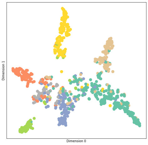
Test set results: loss= 0.7287 accuracy= 0.8240
CPU times: user 8.25 s, sys: 402 ms, total: 8.65 s
Wall time: 4.21 s
3. (DIY) Graph Classification on Collab Dataset
Collab Dataset
it is a large dataset containing many graphs and graph labels.
This dataset is mainly used for graph classification.
COLLAB is a scientific collaboration dataset. A graph corresponds to a researcher’s ego network,
i.e., the researcher and its collaborators are nodes and an edge indicates collaboration between two researchers.
The code is made on pytorch_geometric library.
Why do I use?
pytorch_geometric is very fast despite working on sparse data.
Compared to the Deep GraphLibrary (DGL) 0.1.3, pytorch_geometric trains models up to 15 times faster.
So, I recommend running the code and studying the library.
Reference : https://medium.com/syncedreview/pytorch-geometric-a-fast-pytorch-library-for-dl-a833dff466e5
Prem
pip install torch-scatter torch-sparse torch-cluster torch-spline-conv torch-geometric -f https://data.pyg.org/whl/torch-1.12.0+cu113.htmlLooking in indexes: https://pypi.org/simple, https://us-python.pkg.dev/colab-wheels/public/simple/
Looking in links: https://data.pyg.org/whl/torch-1.12.0+cu113.html
Collecting torch-scatter
Downloading torch_scatter-2.1.1.tar.gz (107 kB)
[2K [90m━━━━━━━━━━━━━━━━━━━━━━━━━━━━━━━━━━━━━━━[0m [32m107.6/107.6 KB[0m [31m3.7 MB/s[0m eta [36m0:00:00[0m
[?25h Preparing metadata (setup.py) ... [?25l[?25hdone
Collecting torch-sparse
Downloading torch_sparse-0.6.17.tar.gz (209 kB)
[2K [90m━━━━━━━━━━━━━━━━━━━━━━━━━━━━━━━━━━━━━━[0m [32m209.2/209.2 KB[0m [31m10.4 MB/s[0m eta [36m0:00:00[0m
[?25h Preparing metadata (setup.py) ... [?25l[?25hdone
Collecting torch-cluster
Downloading torch_cluster-1.6.1.tar.gz (53 kB)
[2K [90m━━━━━━━━━━━━━━━━━━━━━━━━━━━━━━━━━━━━━━━━[0m [32m53.8/53.8 KB[0m [31m1.9 MB/s[0m eta [36m0:00:00[0m
[?25h Preparing metadata (setup.py) ... [?25l[?25hdone
Collecting torch-spline-conv
Downloading torch_spline_conv-1.2.2.tar.gz (25 kB)
Preparing metadata (setup.py) ... [?25l[?25hdone
Collecting torch-geometric
Downloading torch_geometric-2.3.0.tar.gz (616 kB)
[2K [90m━━━━━━━━━━━━━━━━━━━━━━━━━━━━━━━━━━━━━━[0m [32m616.2/616.2 KB[0m [31m25.8 MB/s[0m eta [36m0:00:00[0m
[?25h Installing build dependencies ... [?25l[?25hdone
Getting requirements to build wheel ... [?25l[?25hdone
Preparing metadata (pyproject.toml) ... [?25l[?25hdone
Requirement already satisfied: scipy in /usr/local/lib/python3.9/dist-packages (from torch-sparse) (1.10.1)
Requirement already satisfied: requests in /usr/local/lib/python3.9/dist-packages (from torch-geometric) (2.27.1)
Requirement already satisfied: psutil>=5.8.0 in /usr/local/lib/python3.9/dist-packages (from torch-geometric) (5.9.4)
Requirement already satisfied: jinja2 in /usr/local/lib/python3.9/dist-packages (from torch-geometric) (3.1.2)
Requirement already satisfied: pyparsing in /usr/local/lib/python3.9/dist-packages (from torch-geometric) (3.0.9)
Requirement already satisfied: scikit-learn in /usr/local/lib/python3.9/dist-packages (from torch-geometric) (1.2.2)
Requirement already satisfied: tqdm in /usr/local/lib/python3.9/dist-packages (from torch-geometric) (4.65.0)
Requirement already satisfied: numpy in /usr/local/lib/python3.9/dist-packages (from torch-geometric) (1.22.4)
Requirement already satisfied: MarkupSafe>=2.0 in /usr/local/lib/python3.9/dist-packages (from jinja2->torch-geometric) (2.1.2)
Requirement already satisfied: idna<4,>=2.5 in /usr/local/lib/python3.9/dist-packages (from requests->torch-geometric) (3.4)
Requirement already satisfied: urllib3<1.27,>=1.21.1 in /usr/local/lib/python3.9/dist-packages (from requests->torch-geometric) (1.26.15)
Requirement already satisfied: certifi>=2017.4.17 in /usr/local/lib/python3.9/dist-packages (from requests->torch-geometric) (2022.12.7)
Requirement already satisfied: charset-normalizer~=2.0.0 in /usr/local/lib/python3.9/dist-packages (from requests->torch-geometric) (2.0.12)
Requirement already satisfied: joblib>=1.1.1 in /usr/local/lib/python3.9/dist-packages (from scikit-learn->torch-geometric) (1.1.1)
Requirement already satisfied: threadpoolctl>=2.0.0 in /usr/local/lib/python3.9/dist-packages (from scikit-learn->torch-geometric) (3.1.0)
Building wheels for collected packages: torch-scatter, torch-sparse, torch-cluster, torch-spline-conv, torch-geometric
Building wheel for torch-scatter (setup.py) ... [?25l[?25hdone
Created wheel for torch-scatter: filename=torch_scatter-2.1.1-cp39-cp39-linux_x86_64.whl size=3507043 sha256=c2f0bf45642a83726394a5594e9145f782017baff4117ac6a0a26ecdc38ce660
Stored in directory: /root/.cache/pip/wheels/d5/0c/18/11b4cf31446c5d460543b0fff930fcac3a3f8a785e5c73fb15
Building wheel for torch-sparse (setup.py) ... [?25l[?25hdone
Created wheel for torch-sparse: filename=torch_sparse-0.6.17-cp39-cp39-linux_x86_64.whl size=2746513 sha256=dc5b149df8731c80cb9b8a62f78492502e7788f3d4d6b24745588c74b20ae3c1
Stored in directory: /root/.cache/pip/wheels/f8/43/54/bcb8acdd1109bd1e4c71106747af298d0315cdf3f090b2ae43
Building wheel for torch-cluster (setup.py) ... [?25l[?25hdone
Created wheel for torch-cluster: filename=torch_cluster-1.6.1-cp39-cp39-linux_x86_64.whl size=2077653 sha256=60ccdbefbf1a98a82eeac9797ba687f1e71304af83d41eecf6b030ead8ca57f2
Stored in directory: /root/.cache/pip/wheels/77/5a/b9/b61ba7d7a2e314173db70b38be991ddedc0225a4812bed2dc7
Building wheel for torch-spline-conv (setup.py) ... [?25l[?25hdone
Created wheel for torch-spline-conv: filename=torch_spline_conv-1.2.2-cp39-cp39-linux_x86_64.whl size=523110 sha256=1bc0fc8169a38b61e1da5d10c120f35d63bf2c2c34b30372baa450b41c5f4e51
Stored in directory: /root/.cache/pip/wheels/58/f8/af/928307700e029de11dd581e4a466b4c906bb0764d2d4b591f0
Building wheel for torch-geometric (pyproject.toml) ... [?25l[?25hdone
Created wheel for torch-geometric: filename=torch_geometric-2.3.0-py3-none-any.whl size=909897 sha256=0d7a32ab127edd9c76f32b7dcecd54bf9737c44353daec674686170ecb6acd74
Stored in directory: /root/.cache/pip/wheels/cd/7d/6b/17150450b80b4a3656a84330e22709ccd8dc0f8f4773ba4133
Successfully built torch-scatter torch-sparse torch-cluster torch-spline-conv torch-geometric
Installing collected packages: torch-spline-conv, torch-scatter, torch-sparse, torch-cluster, torch-geometric
Successfully installed torch-cluster-1.6.1 torch-geometric-2.3.0 torch-scatter-2.1.1 torch-sparse-0.6.17 torch-spline-conv-1.2.2from torch_geometric.datasets import TUDataset
from torch_geometric.utils import to_networkx
import torch_geometric.transforms as T
from torch_geometric.utils import degree%%time
def create_one_hot_transform(dataset): # Since the collab dataset does not have a node feature, So I make a node feature using the max_degree value.
max_degree = 0 # I reference that in https://paperswithcode.com/sota/graph-classification-on-collab.
degs = []
for data in dataset:
degs += [degree(data.edge_index[0], dtype=torch.long)]
max_degree = max(max_degree, degs[-1].max().item())
return T.OneHotDegree(max_degree)
def load_dataset():
dataset = TUDataset(root='/tmp/COLLAB', name="COLLAB")
dataset.transform = create_one_hot_transform(dataset)
return dataset
dataset = load_dataset()Downloading https://www.chrsmrrs.com/graphkerneldatasets/COLLAB.zip
Extracting /tmp/COLLAB/COLLAB/COLLAB.zip
Processing...
Done!
CPU times: user 1min 33s, sys: 11.4 s, total: 1min 44s
Wall time: 1min 44sprint()
print(f'Dataset: {dataset}:')
print('====================')
print(f'Number of graphs: {len(dataset)}')
print(f'Number of classes: {dataset.num_classes}')
print(f'Number of features: {dataset.num_features}')
###### One graph #####
data = dataset[0] # Get the first graph object.
print()
print(data)
print('=============================================================')
# Gather some statistics about the first graph.
print(f'Number of nodes: {data.num_nodes}')
print(f'Number of edges: {data.num_edges}')
print(f'Average node degree: {data.num_edges / data.num_nodes:.2f}')
print(f'Contains isolated nodes: {data.contains_isolated_nodes()}')
print(f'Contains self-loops: {data.contains_self_loops()}')
print(f'Is undirected: {data.is_undirected()}')Dataset: COLLAB(5000):
====================
Number of graphs: 5000
Number of classes: 3
Number of features: 492
Data(edge_index=[2, 1980], y=[1], num_nodes=45, x=[45, 492])
=============================================================
Number of nodes: 45
Number of edges: 1980
Average node degree: 44.00
Contains isolated nodes: False
Contains self-loops: False
Is undirected: True# One graph edges
print(data.edge_index)tensor([[ 0, 0, 0, ..., 44, 44, 44],
[ 1, 2, 3, ..., 41, 42, 43]])from torch_geometric.utils import to_networkx
G = to_networkx(data, to_undirected=True)
#It shows one graph of Collab dataset.
plt.figure(figsize=(10, 10))
nx.draw_networkx(G, pos=nx.spring_layout(G, seed=42), with_labels=True, cmap="Set2", width=0.5, node_size=500, node_color='yellow')
plt.axis('off')
plt.tight_layout()
plt.show()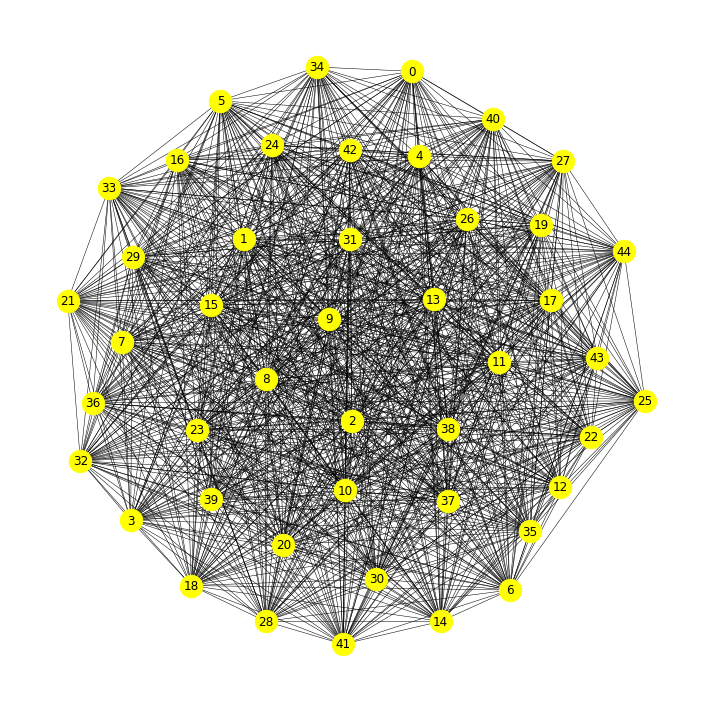
torch.manual_seed(12345)
dataset = dataset.shuffle() # Label data are sequentially located. (0, 1, 2)

# train / valid
train_dataset = dataset[:4000]
valid_dataset = dataset[4000:]

print(f'Number of training graphs: {len(train_dataset)}')
print(f'Number of test graphs: {len(valid_dataset)}')
Number of training graphs: 4000
Number of test graphs: 1000from torch_geometric.data import DataLoader
# Unlike CV and NLP, in graph, DataLoader aggregates node_feature, weight and edge_index from different samples/ graphs into Batches
# So The GNN model needs this “batch” information to know which nodes belong to the same graph within a batch to perform computation.
# Reference : https://towardsdatascience.com/hands-on-graph-neural-networks-with-pytorch-pytorch-geometric-359487e221a8
# Reference : https://pytorch-geometric.readthedocs.io/en/latest/notes/batching.html
train_loader = DataLoader(train_dataset, batch_size=64, shuffle=True)
valid_loader = DataLoader(valid_dataset, batch_size=64, shuffle=False)from torch.nn import Linear
import torch.nn.functional as F
from torch_geometric.nn import GCNConv
from torch_geometric.nn import global_mean_pool
class GCN(torch.nn.Module):
def __init__(self, hidden_channels):
super(GCN, self).__init__()
torch.manual_seed(12345)
self.conv1 = GCNConv(dataset.num_node_features, hidden_channels)
self.conv2 = GCNConv(hidden_channels, hidden_channels)
self.conv3 = GCNConv(hidden_channels, hidden_channels) # When I used one more GCNConv, the performance came out better.
self.lin = Linear(hidden_channels, dataset.num_classes)
def forward(self, x, edge_index, batch):
# 1. Obtain node embeddings
#ipdb.set_trace()
x = self.conv1(x, edge_index)
x = x.relu()
x = self.conv2(x, edge_index)
x = x.relu()
x = self.conv3(x, edge_index)
# 2. Readout layer
x = global_mean_pool(x, batch) # [batch_size, hidden_channels] , for graph classsification
h = x.clone().detach() # for making graph embedding
# 3. Apply a final classifier
x = F.dropout(x, p=0.5, training=self.training)
x = self.lin(x)
return x , hmodel = GCN(hidden_channels=64)
model = model.to(device)
optimizer = torch.optim.Adam(model.parameters(), lr=0.01)
criterion = torch.nn.CrossEntropyLoss()
def train(epoch=None):
model.train()
for data in train_loader: # Iterate in batches over the training dataset.
data = data.to(device)
out, _ = model(data.x, data.edge_index, data.batch) # Perform a single forward pass.
loss = criterion(out, data.y) # Compute the loss.
loss.backward() # Derive gradients.
optimizer.step() # Update parameters based on gradients.
optimizer.zero_grad() # Clear gradients.
print(f'Epoch: {epoch:03d}, Train loss: {loss:.4f}')
def test(loader, visual=False):
model.eval()
correct = 0
for data in loader: # Iterate in batches over the training/test dataset.
data = data.to(device)
out, h = model(data.x, data.edge_index, data.batch)
pred = out.argmax(dim=1) # Use the class with highest probability.
correct += int((pred == data.y).sum()) # Check against ground-truth labels.
if visual == True:
colors = ['#3A3120', '#535D8E', '#BD3430']
color = [ colors[i] for i in data.y.detach().cpu()]
z = TSNE(n_components=2).fit_transform(h.detach().cpu().numpy())
plt.figure(figsize=(10,10))
plt.xticks([])
plt.yticks([])
print(f'Embedding shape: {list(h.shape)}')
plt.scatter(z[:, 0], z[:, 1], s=70, c=color, cmap="Set2")
plt.show()
return correct / len(loader.dataset) # Derive ratio of correct predictions.%%time
################################
for epoch in range(1, 31):
train(epoch)
test_acc = test(valid_loader)
if epoch % 5 == 0:
print(f'Epoch: {epoch:03d}, Test Acc: {test_acc:.4f}')Epoch: 001, Train loss: 0.7195
Epoch: 002, Train loss: 0.4161
Epoch: 003, Train loss: 0.4312
Epoch: 004, Train loss: 0.4805
Epoch: 005, Train loss: 0.3761
Epoch: 005, Test Acc: 0.7810
Epoch: 006, Train loss: 0.6026
Epoch: 007, Train loss: 0.3423
Epoch: 008, Train loss: 0.4011
Epoch: 009, Train loss: 0.3502
Epoch: 010, Train loss: 0.3265
Epoch: 010, Test Acc: 0.7960
Epoch: 011, Train loss: 0.3840
Epoch: 012, Train loss: 0.5217
Epoch: 013, Train loss: 0.4022
Epoch: 014, Train loss: 0.3394
Epoch: 015, Train loss: 0.3952
Epoch: 015, Test Acc: 0.8010
Epoch: 016, Train loss: 0.3260
Epoch: 017, Train loss: 0.5382
Epoch: 018, Train loss: 0.4368
Epoch: 019, Train loss: 0.2666
Epoch: 020, Train loss: 0.2966
Epoch: 020, Test Acc: 0.7890
Epoch: 021, Train loss: 0.3952
Epoch: 022, Train loss: 0.2110
Epoch: 023, Train loss: 0.2415
Epoch: 024, Train loss: 0.1759
Epoch: 025, Train loss: 0.2747
Epoch: 025, Test Acc: 0.8190
Epoch: 026, Train loss: 0.2576
Epoch: 027, Train loss: 0.3284
Epoch: 028, Train loss: 0.4078
Epoch: 029, Train loss: 0.2570
Epoch: 030, Train loss: 0.2867
Epoch: 030, Test Acc: 0.8110
CPU times: user 2min, sys: 345 ms, total: 2min
Wall time: 1min 3stest(valid_loader, visual=True) # t-SNEEmbedding shape: [64, 64]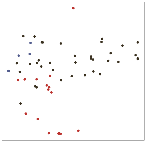
Embedding shape: [64, 64]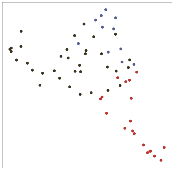
Embedding shape: [64, 64]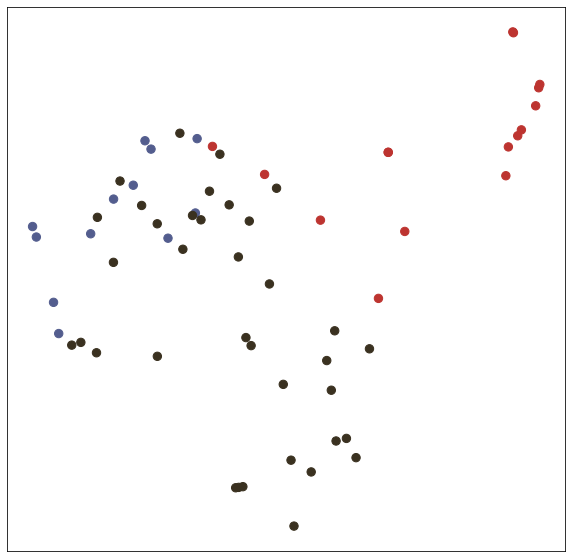
Embedding shape: [64, 64]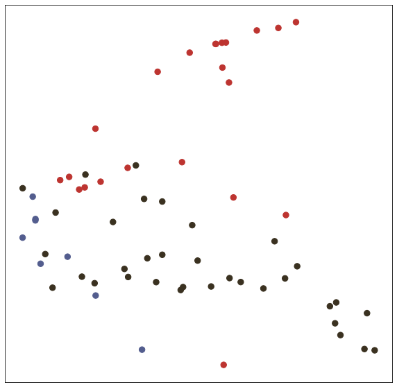
Embedding shape: [64, 64]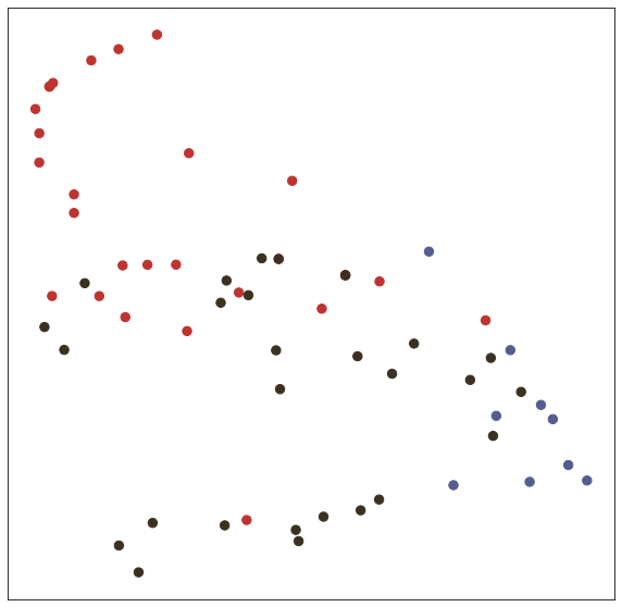
Embedding shape: [64, 64]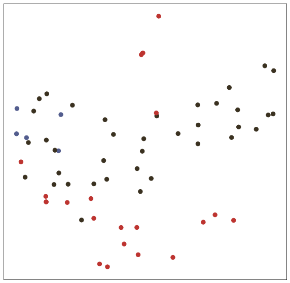
Embedding shape: [64, 64]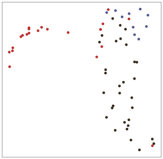
Embedding shape: [64, 64]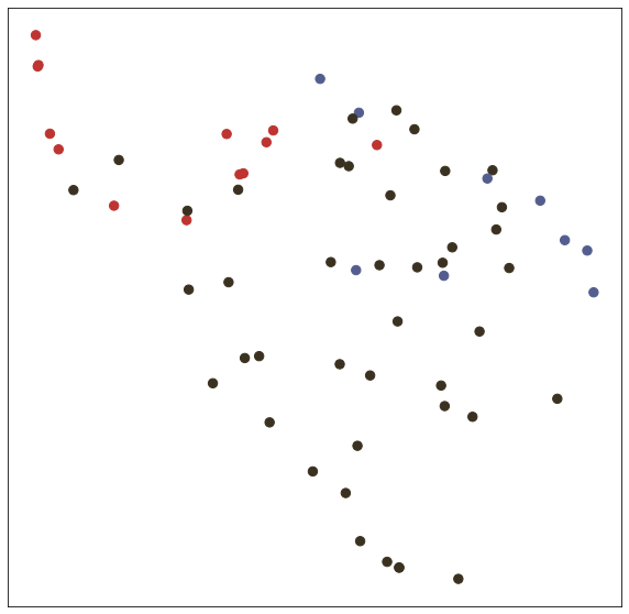
Embedding shape: [64, 64]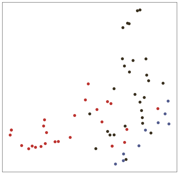
Embedding shape: [64, 64]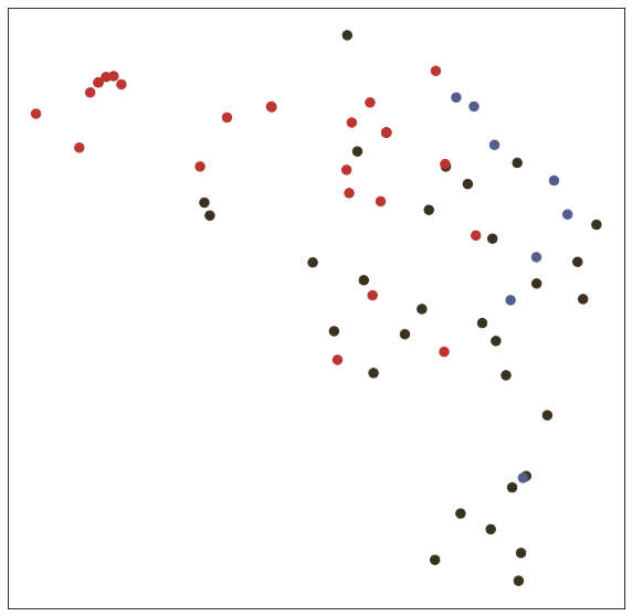
Embedding shape: [64, 64]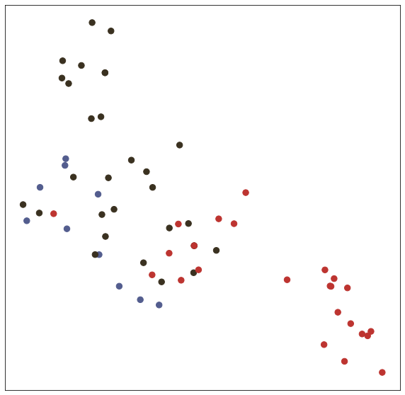
Embedding shape: [64, 64]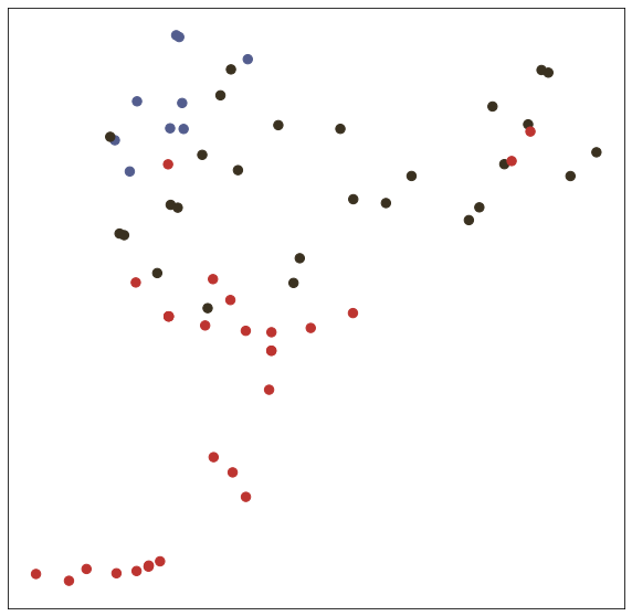
Embedding shape: [64, 64]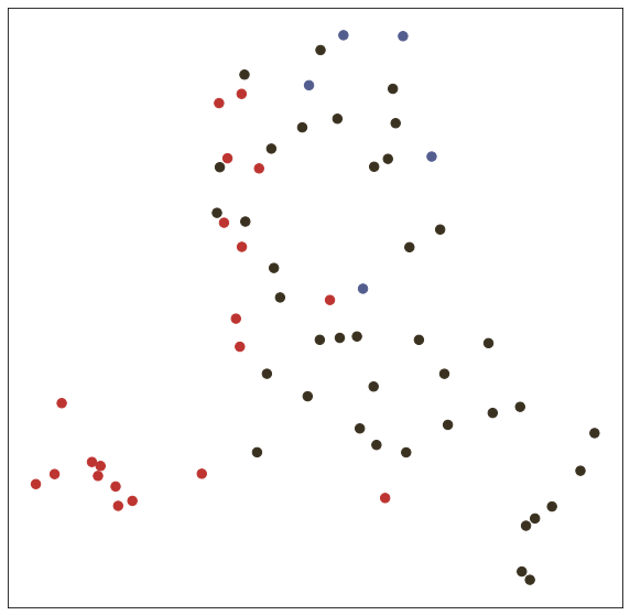
Embedding shape: [64, 64]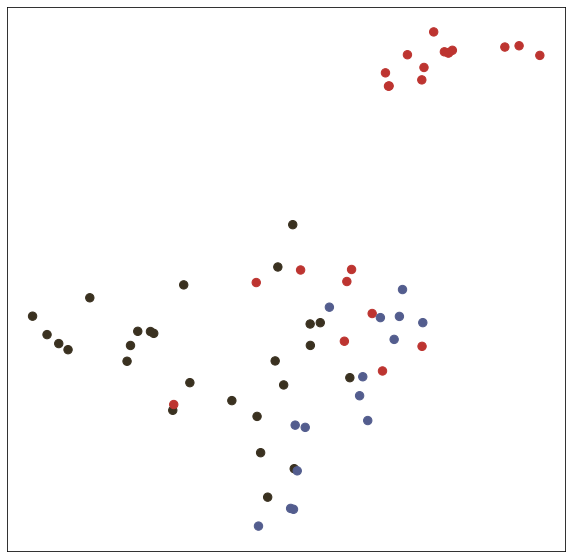
Embedding shape: [64, 64]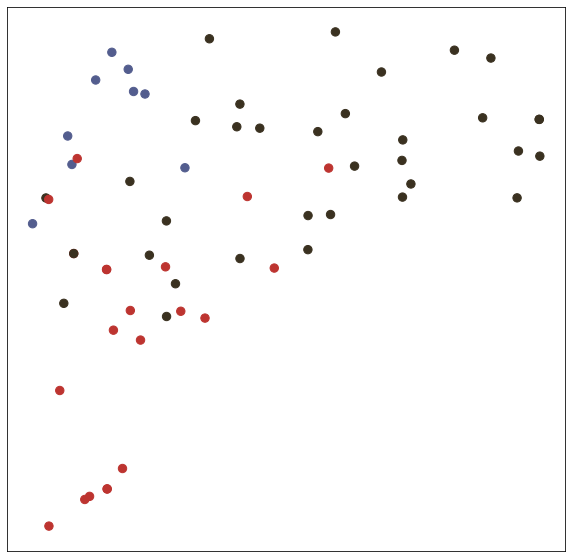
Embedding shape: [40, 64]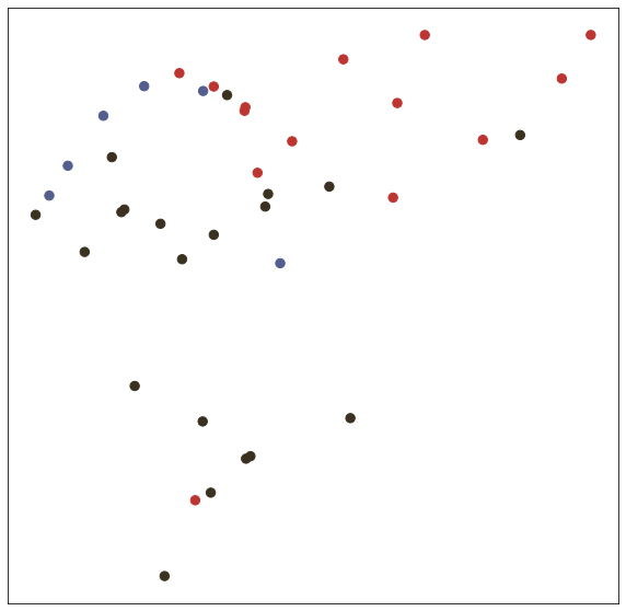
0.811Reference
Thomas N. Kipf, Max Welling, Semi-Supervised Classification with Graph Convolutional Networks (ICLR 2017)
http://tkipf.github.io/graph-convolutional-networks/
https://relational.fit.cvut.cz/dataset/CORA
https://paperswithcode.com/sota/graph-classification-on-collab
https://pytorch-geometric.readthedocs.io/en/latest/notes/batching.html
https://medium.com/syncedreview/pytorch-geometric-a-fast-pytorch-library-for-dl-a833dff466e5
https://towardsdatascience.com/hands-on-graph-neural-networks-with-pytorch-pytorch-geometric-359487e221a8
https://paperswithcode.com/sota/node-classification-on-cora
https://graphsandnetworks.com/the-cora-dataset/
https://github.com/tkipf/pygcn
https://pytorch-geometric.readthedocs.io/en/latest/
https://colab.research.google.com/drive/1I8a0DfQ3fI7Njc62__mVXUlcAleUclnb?usp=sharing
http://networkrepository.com/COLLAB.php
Reference
- AI504: Programming for AI Lecture at KAIST AI