[AI504] Practice 02: Basic Machine Learning

Today's Practice Topics

1. Data Plotting

2. Generating Samples

3. Regression (Overfitting, underfitting)

4. Data Loading

5. Classification

import numpy as np
from matplotlib import pyplot as plt # provide a lot of API for you to draw things
import sklearn

Matplotlib Example

plt.plot([1,2,3], [3,2,1]) # usual line plot (the line that go through these three dots)
plt.scatter([1,2,3], [3,2,1]) # dots
plt.show()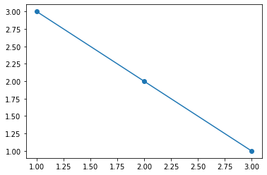

# X and Y should be a list
# x_sample and y_sample are dots for drawing scatter plot
def draw_plot(X, Y, x_sample, y_sample):
    for i in range(len(X)):
        plt.plot(X[i], Y[i])
    plt.scatter(x_sample, y_sample)
    plt.xlabel('x')
    plt.ylabel('y')
    plt.axhline(0, color='black')
    plt.axvline(0, color='black')
    plt.show()

Drawing a function

함수를 visualize 하는 기본적인 방법
1. define function
2. define bunch of x that you want to feed into the function typically using linspace
3. you get corresponding output y
4. call plot function
5. visualize

# define function which is third order polynomial
foo = lambda x: -(2/7*x**3-9/2*x**2+15*x-10.)
# linspace(beginning, end, how many points you want between beginning and end)
x_line = np.linspace(0, 10, 100)

# Quiz: Draw the function foo using x_line
# feed x_line vector into function foo so that we can get a lot of y
y_line = foo(x_line)
plt.plot(x_line, y_line)
plt.show()

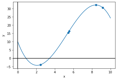
# Quiz: Sample 5 points of foo in the domain [0, 10] and visualize with draw_plot
# when we sample, we typically use uniform function
x_sample = np.random.uniform(0,10,5)
y_sample = foo(x_sample)
draw_plot([x_line], [y_line], x_sample, y_sample) # x_line and y_line should be a list

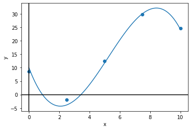
# Quiz: Sample 5 points of foo in the domain [0, 10] with Gaussian noise where mu=0, sigma=0.1 and visualize.
sample_size = 5
x_sample = np.linspace(0, 10, sample_size)
np.random.seed(200)
y_sample = foo(x_sample) + np.random.normal(loc=0, scale=1, size=sample_size)
draw_plot([x_line], [y_line], x_sample, y_sample)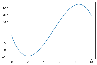

Linear Regression

from sklearn.linear_model import LinearRegression

# Defining a linear regression model.
lr = LinearRegression()

# Training the linear regression model.
# None을 붙이는 이유는 2D array를 원하기 때문이다. fit function is expecting x to be a matrix
# that is why we increase 1 dimension to make it into matrix.
# x_sample is a vector, a 1 dimensional array
lr.fit(x_sample[:, None], y_sample)

# Coefficient of Determination (i.e. R^2, R Squared)
# This is how we evaluate the performance of regression function.
r2 = lr.score(x_sample[:, None], y_sample) # evaluation metric
print("R^2:%f" % r2)

# Predicting a single data point.
y_hat = lr.predict(x_sample[:, None][0][None, :]) # 1 by 1 shape
print(x_sample)
print(y_sample)
print(y_hat)

# Quiz: Calculate Mean Squared Error using x_sample and y_sample and lr.predict()
y_hat = lr.predict(x_sample[:, None])
mse = ((y_sample-y_hat)**2).sum() / x_sample.size
print(mse)

# Quiz: Use x_line, lr.predict() and draw_plot to visualize the linear regression model,
#       in comparison with the original function foo.
y_pred_line = lr.predict(x_line[:, None])
# we use list because we want to draw multiple plot on the same plane
draw_plot([x_line, x_line], [y_line, y_pred_line], x_sample, y_sample)

R^2:0.632018
[ 0.   2.5  5.   7.5 10. ]
[ 8.54905175 -1.92833258 12.49759344 29.84154743 24.64718052]
[1.9281806]
47.64601908459361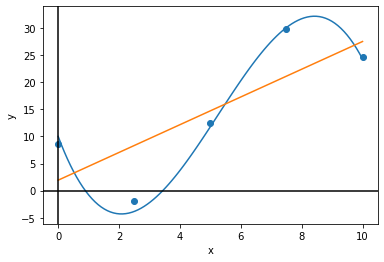

Polynomial Regression

sklearn에 PolynomialRegression Library는 없다.
그래서 feature를 polynomial function을 사용하여 higher order space로 바꾸면 feature가 polynomial feature가 되니까 여기에 LinearRegression을 fitting한다. 이렇게 하여 sklearn setting에서 PolynomialRegression을 구현한다.

original feature와 degree를 주면 PolynomialFeatures function은 주어진 feature를 원하는 polynomial order에 맞게 변환한다.

from sklearn.preprocessing import PolynomialFeatures
from sklearn.linear_model import Ridge

# Defining a polynomial feature transformer.
poly = PolynomialFeatures(degree=6)

# Transform the original features to polynomial features.
x_sample_poly = poly.fit_transform(x_sample[:, None]) # transform into second order polynomial function

# That is what PolynomialFeatures do
#print(x_sample[:, None])
#print(x_sample_poly)

# Train a linear regression model using the polynomial features.
pr = LinearRegression().fit(x_sample_poly, y_sample)
x_poly_line = poly.fit_transform(x_line[:, None])

# Quiz: Visualize the polynomial regression model, in comparison with foo.
pr_line = pr.predict(x_poly_line)
#print(pr_line)

rr = Ridge(alpha=50.0).fit(x_sample_poly, y_sample)
rr_line = rr.predict(x_poly_line)
draw_plot([x_line, x_line, x_line], [y_line, pr_line, rr_line], x_sample, y_sample)
# Quiz: What happens if you increase/decrease the degree of the polynomial?
# degree 1 and 2 : underfitting
# degree 3 and 4 : perfect fitting and acceptable
# degree 5 and over : overfitting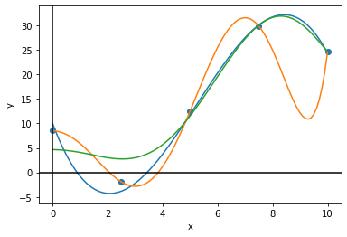

Remedy for handling overfitting
1. Regularization(There were L2 Regularization and L1 Regularization)
2. increase number of samples (not always easy to increase sample because it usually needs human annotation)

dataset size를 많이 늘릴 수 없는 상황이라면 regularization이 좋은 선택이 될 수 있다.

L2 Regularization term을 높이면 movement를 restricting하게 되어 polynomial behavior가 약해진다.

Iris Dataset

data_path = './iris.data'
X = []
y = []
with open(data_path, 'r') as fid:
    count = 0
    for line in fid:
        #print(line.strip())
        words = line.split(',')
        if len(words) == 5 :
          features = list(map(float, words[:4]))
          X.append(features)
          if words[4] == 'Iris-setosa\n' :
            y.append(0)
          elif words[4] == 'Iris-versicolor\n' :
            y.append(1)
          elif words[4] == 'Iris-virginica\n' :
            y.append(2)

X = np.array(X)
y = np.array(y)
print(X)
print(y)
# Quiz: Fill the above for loop to load the data into X and y.

[[5.1 3.5 1.4 0.2]
 [4.9 3.  1.4 0.2]
 [4.7 3.2 1.3 0.2]
 [4.6 3.1 1.5 0.2]
 [5.  3.6 1.4 0.2]
 [5.4 3.9 1.7 0.4]
 [4.6 3.4 1.4 0.3]
 [5.  3.4 1.5 0.2]
 [4.4 2.9 1.4 0.2]
 [4.9 3.1 1.5 0.1]
 [5.4 3.7 1.5 0.2]
 [4.8 3.4 1.6 0.2]
 [4.8 3.  1.4 0.1]
 [4.3 3.  1.1 0.1]
 [5.8 4.  1.2 0.2]
 [5.7 4.4 1.5 0.4]
 [5.4 3.9 1.3 0.4]
 [5.1 3.5 1.4 0.3]
 [5.7 3.8 1.7 0.3]
 [5.1 3.8 1.5 0.3]
 [5.4 3.4 1.7 0.2]
 [5.1 3.7 1.5 0.4]
 [4.6 3.6 1.  0.2]
 [5.1 3.3 1.7 0.5]
 [4.8 3.4 1.9 0.2]
 [5.  3.  1.6 0.2]
 [5.  3.4 1.6 0.4]
 [5.2 3.5 1.5 0.2]
 [5.2 3.4 1.4 0.2]
 [4.7 3.2 1.6 0.2]
 [4.8 3.1 1.6 0.2]
 [5.4 3.4 1.5 0.4]
 [5.2 4.1 1.5 0.1]
 [5.5 4.2 1.4 0.2]
 [4.9 3.1 1.5 0.1]
 [5.  3.2 1.2 0.2]
 [5.5 3.5 1.3 0.2]
 [4.9 3.1 1.5 0.1]
 [4.4 3.  1.3 0.2]
 [5.1 3.4 1.5 0.2]
 [5.  3.5 1.3 0.3]
 [4.5 2.3 1.3 0.3]
 [4.4 3.2 1.3 0.2]
 [5.  3.5 1.6 0.6]
 [5.1 3.8 1.9 0.4]
 [4.8 3.  1.4 0.3]
 [5.1 3.8 1.6 0.2]
 [4.6 3.2 1.4 0.2]
 [5.3 3.7 1.5 0.2]
 [5.  3.3 1.4 0.2]
 [7.  3.2 4.7 1.4]
 [6.4 3.2 4.5 1.5]
 [6.9 3.1 4.9 1.5]
 [5.5 2.3 4.  1.3]
 [6.5 2.8 4.6 1.5]
 [5.7 2.8 4.5 1.3]
 [6.3 3.3 4.7 1.6]
 [4.9 2.4 3.3 1. ]
 [6.6 2.9 4.6 1.3]
 [5.2 2.7 3.9 1.4]
 [5.  2.  3.5 1. ]
 [5.9 3.  4.2 1.5]
 [6.  2.2 4.  1. ]
 [6.1 2.9 4.7 1.4]
 [5.6 2.9 3.6 1.3]
 [6.7 3.1 4.4 1.4]
 [5.6 3.  4.5 1.5]
 [5.8 2.7 4.1 1. ]
 [6.2 2.2 4.5 1.5]
 [5.6 2.5 3.9 1.1]
 [5.9 3.2 4.8 1.8]
 [6.1 2.8 4.  1.3]
 [6.3 2.5 4.9 1.5]
 [6.1 2.8 4.7 1.2]
 [6.4 2.9 4.3 1.3]
 [6.6 3.  4.4 1.4]
 [6.8 2.8 4.8 1.4]
 [6.7 3.  5.  1.7]
 [6.  2.9 4.5 1.5]
 [5.7 2.6 3.5 1. ]
 [5.5 2.4 3.8 1.1]
 [5.5 2.4 3.7 1. ]
 [5.8 2.7 3.9 1.2]
 [6.  2.7 5.1 1.6]
 [5.4 3.  4.5 1.5]
 [6.  3.4 4.5 1.6]
 [6.7 3.1 4.7 1.5]
 [6.3 2.3 4.4 1.3]
 [5.6 3.  4.1 1.3]
 [5.5 2.5 4.  1.3]
 [5.5 2.6 4.4 1.2]
 [6.1 3.  4.6 1.4]
 [5.8 2.6 4.  1.2]
 [5.  2.3 3.3 1. ]
 [5.6 2.7 4.2 1.3]
 [5.7 3.  4.2 1.2]
 [5.7 2.9 4.2 1.3]
 [6.2 2.9 4.3 1.3]
 [5.1 2.5 3.  1.1]
 [5.7 2.8 4.1 1.3]
 [6.3 3.3 6.  2.5]
 [5.8 2.7 5.1 1.9]
 [7.1 3.  5.9 2.1]
 [6.3 2.9 5.6 1.8]
 [6.5 3.  5.8 2.2]
 [7.6 3.  6.6 2.1]
 [4.9 2.5 4.5 1.7]
 [7.3 2.9 6.3 1.8]
 [6.7 2.5 5.8 1.8]
 [7.2 3.6 6.1 2.5]
 [6.5 3.2 5.1 2. ]
 [6.4 2.7 5.3 1.9]
 [6.8 3.  5.5 2.1]
 [5.7 2.5 5.  2. ]
 [5.8 2.8 5.1 2.4]
 [6.4 3.2 5.3 2.3]
 [6.5 3.  5.5 1.8]
 [7.7 3.8 6.7 2.2]
 [7.7 2.6 6.9 2.3]
 [6.  2.2 5.  1.5]
 [6.9 3.2 5.7 2.3]
 [5.6 2.8 4.9 2. ]
 [7.7 2.8 6.7 2. ]
 [6.3 2.7 4.9 1.8]
 [6.7 3.3 5.7 2.1]
 [7.2 3.2 6.  1.8]
 [6.2 2.8 4.8 1.8]
 [6.1 3.  4.9 1.8]
 [6.4 2.8 5.6 2.1]
 [7.2 3.  5.8 1.6]
 [7.4 2.8 6.1 1.9]
 [7.9 3.8 6.4 2. ]
 [6.4 2.8 5.6 2.2]
 [6.3 2.8 5.1 1.5]
 [6.1 2.6 5.6 1.4]
 [7.7 3.  6.1 2.3]
 [6.3 3.4 5.6 2.4]
 [6.4 3.1 5.5 1.8]
 [6.  3.  4.8 1.8]
 [6.9 3.1 5.4 2.1]
 [6.7 3.1 5.6 2.4]
 [6.9 3.1 5.1 2.3]
 [5.8 2.7 5.1 1.9]
 [6.8 3.2 5.9 2.3]
 [6.7 3.3 5.7 2.5]
 [6.7 3.  5.2 2.3]
 [6.3 2.5 5.  1.9]
 [6.5 3.  5.2 2. ]
 [6.2 3.4 5.4 2.3]
 [5.9 3.  5.1 1.8]]
[0 0 0 0 0 0 0 0 0 0 0 0 0 0 0 0 0 0 0 0 0 0 0 0 0 0 0 0 0 0 0 0 0 0 0 0 0
 0 0 0 0 0 0 0 0 0 0 0 0 0 1 1 1 1 1 1 1 1 1 1 1 1 1 1 1 1 1 1 1 1 1 1 1 1
 1 1 1 1 1 1 1 1 1 1 1 1 1 1 1 1 1 1 1 1 1 1 1 1 1 1 2 2 2 2 2 2 2 2 2 2 2
 2 2 2 2 2 2 2 2 2 2 2 2 2 2 2 2 2 2 2 2 2 2 2 2 2 2 2 2 2 2 2 2 2 2 2 2 2
 2 2]

#from sklearn.datasets import load_iris
#X, y = load_iris(return_X_y = True)

Train Test Split

from sklearn.model_selection import train_test_split
X_train, X_test, y_train, y_test = train_test_split(X, y, test_size=0.20, random_state=0)

Classifiers

Logistic Regression은 binary classifier이지만 Multiclass setting으로 만들 수 있다.

Pattern of how to use sklearn
1. instantiate a class with some hyperparameters or the options defined
2. feed it
3. score it or predict it

from sklearn.linear_model import LogisticRegression
logistic = LogisticRegression(random_state=1234)
# 앞 2개의 column만 이용한다. limiting capacity of the model and trying to make it underfitting so it doesn't perfectly solve the problem
logistic.fit(X_train[:, :2], y_train)
# 세 class가 동일하게 50개씩 있으므로 accuracy를 measure로 사용하기 좋다.
#logistic.score(X_train[:, :2], y_train)
logistic.score(X_test[:, :2], y_test)

# Quiz: Import Support Vector Machine, then train SVM
from sklearn.svm import SVC
svc = SVC(C=1.0, kernel='linear')
svc.fit(X_train[:, :2], y_train)

# Quiz: Import Decision Tree, then train DT
from sklearn.tree import DecisionTreeClassifier as DTC
tree = DTC(max_depth=3, random_state=1234)
tree.fit(X_train[:,:2], y_train)
# max_depth를 늘릴수록 model의 capacity를 늘린다. polynomial order를 늘리는 것과 같은 역할을 한다.
# LogisticRegression, SVM, DT 모두 class 수가 여러개인 것을 알고 Multiclass classifier로 자동으로 변환한다.

DecisionTreeClassifier(max_depth=3, random_state=1234)

# Quiz: Use the model's predict() to calculate the test accuracy.
y_svc = svc.predict(X_test[:,:2])
#print(y_svc)
#print((y_test == y_svc).mean())
print(logistic.score(X_test[:,:2], y_test))
print(svc.score(X_test[:,:2], y_test))
print(tree.score(X_test[:,:2], y_test))

0.7333333333333333
0.7333333333333333
0.6

# Quiz: Use various model options, features, and the score() fuction to compare performance.

y_logistic = logistic.predict(X_test[:,:2])
y_svc = svc.predict(X_test[:,:2])
y_tree = tree.predict(X_test[:,:2])
# Quiz: Can you draw four scatterplots for each model's predictions and the true labels? (Example shown below)
plt.figure(figsize=(20,5))

plt.subplot(141)
plt.title('Logistic Regression')
plt.scatter(X_test[:,0], X_test[:,1], c=y_logistic)

plt.subplot(142)
plt.title('SVM')
plt.scatter(X_test[:,0], X_test[:,1], c=y_svc)

plt.subplot(143)
plt.title('Decision Tree')
plt.scatter(X_test[:,0], X_test[:,1], c=y_tree)

plt.subplot(144)
plt.title('Ground Truth')
plt.scatter(X_test[:,0], X_test[:,1], c=y_test)

plt.show()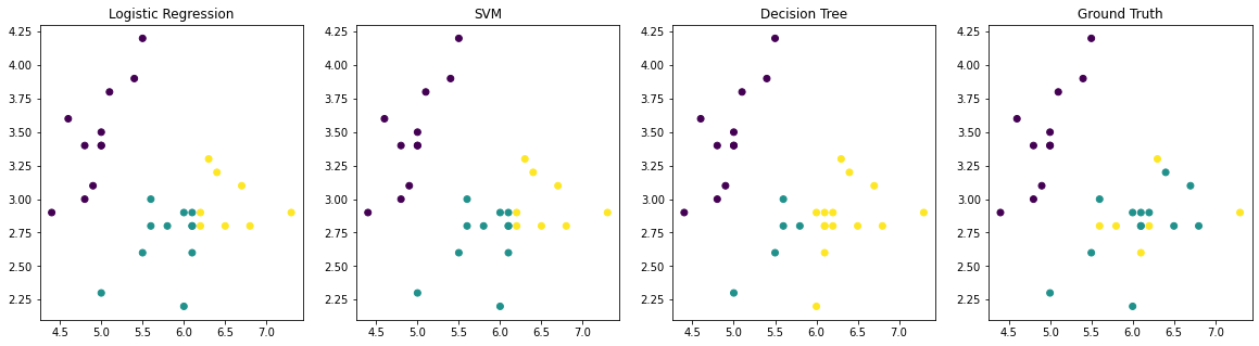

# Drawing the decision boundary of each model. (code by SungMin Kim)
plt.figure(figsize=(20,5))

plt.subplot(141)
plt.title('Ground Truth')
plt.scatter(X_test[:, 0], X_test[:, 1], c=y_test)


plt.subplot(142)
plt.title('Logistic Regression')
plt.scatter(X_test[:, 0], X_test[:, 1], c=y_logistic)

grid_size = 500
A, B = np.meshgrid(np.linspace(X[:, 0].min(), X[:, 0].max(), grid_size),
                   np.linspace(X[:, 1].min(), X[:, 1].max(), grid_size))
C = logistic.predict( np.hstack([A.reshape(-1, 1), B.reshape(-1, 1)]) ).reshape(grid_size, grid_size)
plt.contourf(A, B, C, alpha=0.3, cmap=plt.cm.rainbow)


plt.subplot(143)
plt.title('SVM')
plt.scatter(X_test[:, 0], X_test[:, 1], c=y_svc)

grid_size = 500
A, B = np.meshgrid(np.linspace(X[:, 0].min(), X[:, 0].max(), grid_size),
                   np.linspace(X[:, 1].min(), X[:, 1].max(), grid_size))
C = svc.predict( np.hstack([A.reshape(-1, 1), B.reshape(-1, 1)]) ).reshape(grid_size, grid_size)
plt.contourf(A, B, C, alpha=0.3, cmap=plt.cm.rainbow)


plt.subplot(144)
plt.title('Decision Tree')
plt.scatter(X_test[:, 0], X_test[:, 1], c=y_tree)

grid_size = 500
A, B = np.meshgrid(np.linspace(X[:, 0].min(), X[:, 0].max(), grid_size),
                   np.linspace(X[:, 1].min(), X[:, 1].max(), grid_size))
C = tree.predict( np.hstack([A.reshape(-1, 1), B.reshape(-1, 1)]) ).reshape(grid_size, grid_size)
plt.contourf(A, B, C, alpha=0.3, cmap=plt.cm.rainbow)


plt.show()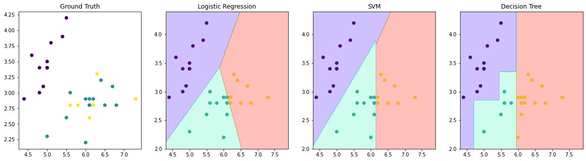

Reference

• AI504: Programming for AI Lecture at KAIST AI