[AI504] Class 02: Basic Machine Learning

Machine Learning Categories

🔗 Supervised Learning

• input x를 output y로 mapping하는 function을 학습한다.
• input과 output이 있는 것은 모두 supervised learning이라고 볼 수 있다.
• Ex. Image classification, French-English translation, Image captioning

🔗 Unsupervised Learning

• data X의 distribution/manifold function을 학습한다.
• 오직 data만 필요하고, label은 필요하지 않다.
• Ex. Clustering, Low-rank matrix factorization, Kernel density estimation

🔗 Reinforcement Learning

• 세 개의 component가 있다.
  • environment E
  • a set of actions A
  • (long-term)reward R
• agent/machine이 E에서 지내면서 A를 수행한다. 그리고 R을 받는다. Reinforcement Learning은 R을 maximize하는 function을 학습하는 것이다.
• Ex. Go, Atari, Self-driving car
• ⭐️ data는 없다.

셋 다 learning이 붙는다. 함수/모델을 학습하기 때문이다. data를 사용하여 함수/모델을 학습한다. 그래서 statistical machine learning이라고 부른다.

generative models와 self-supervised learning는 선이 약간 애매하다.

<Example>
BERT : Labels come from datas. Training sample을 준비하면, 사람이 그것을 수동으로 labeling할 필요가 없다.
Supervised Learning에서는 주로 label은 human annotation을 통해 얻어진다.

(Reinforcement Learning은 제외하고 Supervised Learning과 Unsupervised Learning으로 분류하는 경우도 있다.)

Optimization

• Objective function이라고 불리는 goal을 달성하기 위하여 model f(x; θ)에서 parameter θ를 training하는 것이다. Function/model의 behavior를 결정하는 θ를 tuning/adjusting하여 우리의 model이 의도한대로 행동할 수 있는 최적의 θ를 얻는다.
• θ만 tuning/adjusting하여 Y'을 최대한 Y와 가까워지도록 즉, loss(y, f(x; θ))을 최소화하는 θ를 찾는 것이 optimization이다.
• loss(y, f(x; θ))는 주로 complex, non-convex function이므로 analytical solution이 없다.

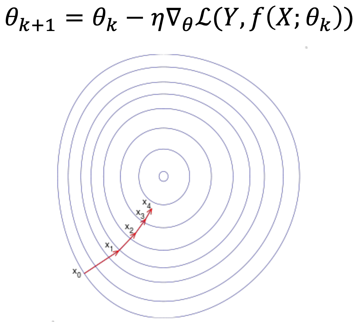
💡 Numerical method 사용 : 더 나은 θ를 반복적으로 찾는다.

• non-convex function에서 numerical method의 문제 : solution이 initial point에 따라 결정된다/바뀐다.

<정리>
Data X와 Y, 그리고 θ에 의해 behavior가 결정되는 function/model이 있을때,
- loss function을 정의하고
- 목표를 달성하기 위해 loss function을 minimize하고싶다.
그러기 위해서는,
- 먼저 task를 수행하기 위한 알맞은 loss function을 선택해야하고
- loss function을 minimize하는 단 하나의 방법인, parameter θ를 optimize해야한다.

Gradient Descent

• Training set에 있는 모든 sample에 대해 average gradient를 구한다.

Stochastic Gradient Descent

• Training data의 subset(minibatch)을 이용하여 true gradient를 approximate한다.
• Modern deep learning은 SGD 기반이다. Minibatch gradient descent를 사용한다.
• True SGD는 오직 하나의 sample을 이용하여 gradient를 구하고 parameter를 update한다.

❓SGD를 사용하는 이유

• Training data가 너무 커서 시간비용과 공간비용이 매우 크다.
• 가끔 smaller batch-size가 suboptimal minimum을 피하는 데 도움을 준다.
  • minibatch를 쓸때마다 loss surface의 형태가 조금씩 바뀌기 때문이다.
• 만약 minibatch가 training samples로부터 I.I.D 하다면, SGD를 통해 얻는 parameter, solution이 GD를 통해 얻은 parameter, solution과 같다는 이론적 보장이 있다.
  • train set에서 minibatch가 random하게 sample되면 이것이 I.I.D하게 minibatch를 sample하는 것이다.

Evaluation

❓언제 SGD를 stop할 지 어떻게 알 수 있을까?
💡Train model/optimize parameter 하는 동안, every 100 iter or 1000 iter 마다 evaulation metrics를 사용하여 모델의 성능을 평가한다.

• Popular Evaluation Metrics
  • Accuracy
  • Area under the ROC (AUROC)
    • task가 inbalance class 일때, positive가 negative에 비해 매우 작을 때 주로 사용한다.
  • Precision & Recall
  • BLEU Score
  • Perplexity
  • FID Score

Train & Validation & Test

전체 dataset을 세 개의 set으로 나눈다.

• Training set
  • Optimize parameter/ train model할 때 사용
• Validation set
  • Optimization process를 언제 stop할지 알기 위해 필요하다.
  • Model이 overfitting되는 것을 막는데 사용된다.
• Test set
  • Optimization process에서 한번도 못보고 사용도 안한다.
  • Unseen data에 대해서 generalize되었는지 final model에 대한 평가를 할 때, test performance를 얻는데 사용된다.

N-fold Cross Validation

• Multiple test set을 가질 수 있다. dataset이 매우 작으면, test set에 대한 결과 performance에 신뢰가 가지 않을 수 있는데, unseen test set에 대해 모델을 평가할 수 있는 multiple chance를 얻음으로써 분산이 적어지고 결과 performance에 믿음이 간다.
• Modern deep learning에는 자주 쓰이지 않는다. 왜냐하면 dataset이 매우 크기 때문에 이미 representative test set이라고 믿을 수 있고, 모델의 true performance를 충분히 estimate할 수 있다. test 여러번 하기에도 시간, 전기 비용이 크다.

Overfitting & Underfitting

• Data complexity VS model capacity
  
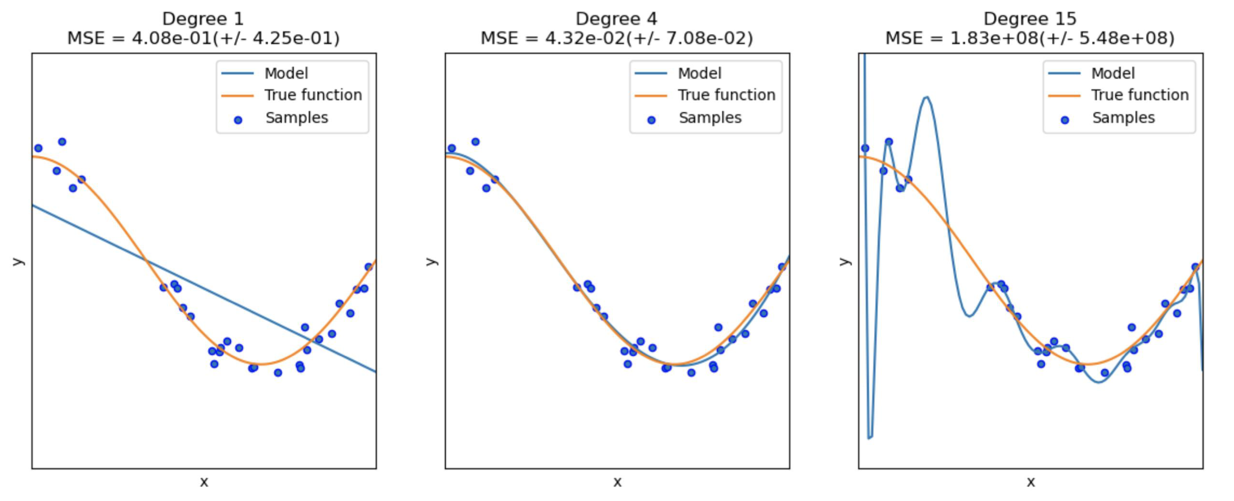
• function의 power를 증가시키면, 주어진 train set에는 더 잘 fit된다.
• model의 power가 너무 크면, train sample의 작은 noise에도 매우 민감해져서 overfitting 하게 된다. 그래서 test samples(unseen data)에는 generalize되지 않는다.

❓model이 overfitting, underfitting된 것을 어떻게 알까?

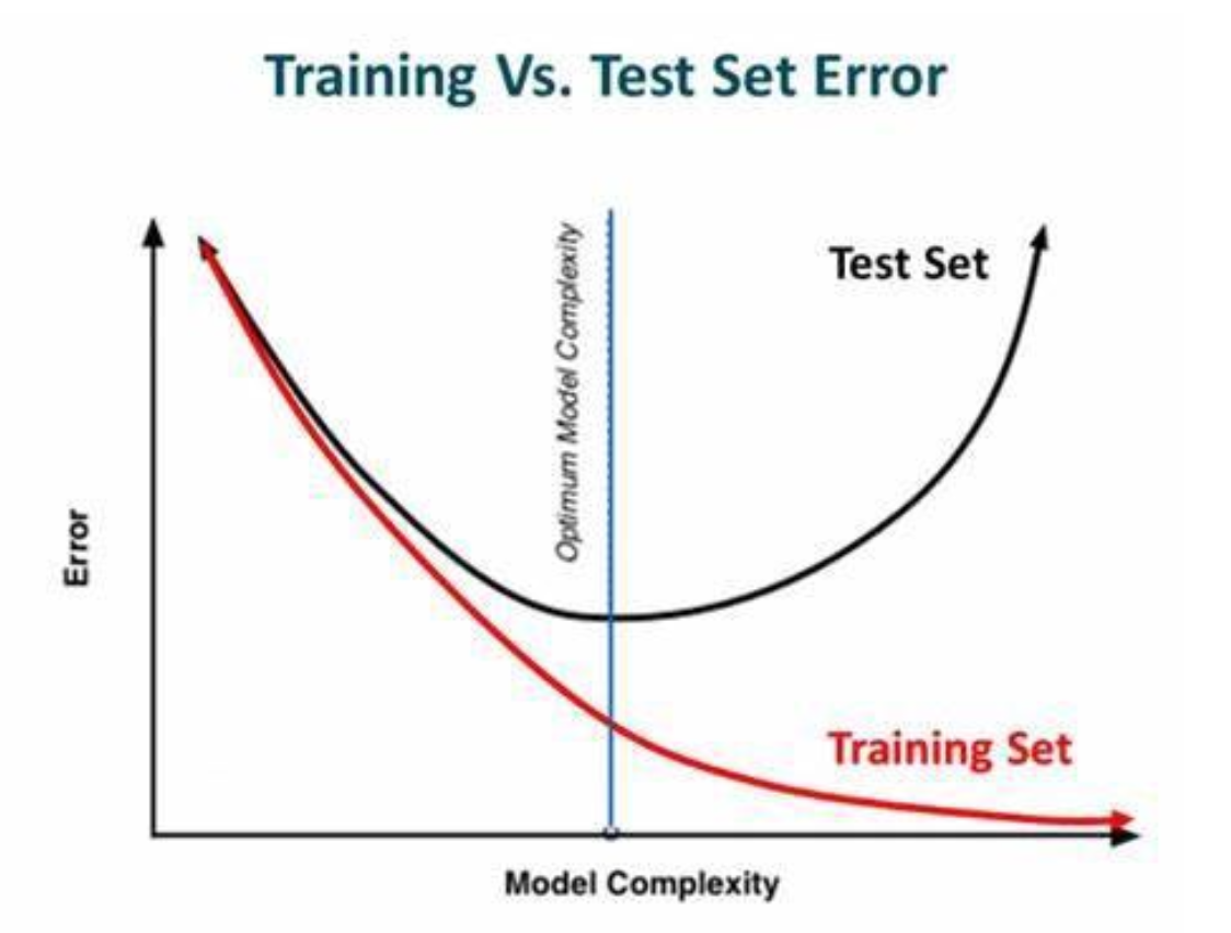
• 언제 validation performance가 감소하기 시작하는지 보고 그때 training process를 멈춘다.

💡Underfitting Remedies

• Complexify model/increase capacity of the model
• Add more features
• Train/optimize longer

💡Overfitting Remedies

• Regularize
• Get more data <- 항상 좋은 해결책이지만 human annotation이 들어가야 하기 때문에 쉽지 않다.

Curse of Dimensionality

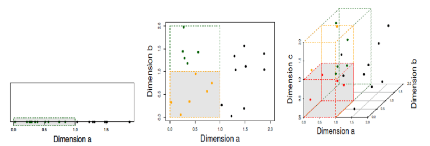
• feature의 수가 linear하게 증가될 때, model은 space를 채우기 위해 exponential하게 증가된 수의 data를 필요로 한다. 그래야 적절한 decision boundary를 그릴 수 있다.
• deep learning, 특히 NLP에서도 역할을 한다. 너무 많은 word를 사용하고 싶어하지 않는다.
• linear algebra 측면에서도, linear equation 수에 비해 너무 많은 variable(feature)가 있으면, 많은 solution이 나올 수 있다.

Regularization

• model의 자유를 제한한다. Hypothesis space를 축소한다.
• model이 급격한 behavior를 보이는 오직 가능한 한 이유는, coefficient 또는 weight가 매우 크기 때문이다. 그래서 model이 smoothier behavior를 보이게 하기 위해 regularization을 사용한다.
• L2 regularization
  
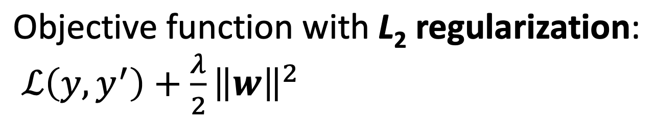
  w : weight vecters (Ex. 15차원 vector)
  • 추가 하나의 term을 loss function에 더한다. loss를 minimizing하면서 weight vectors의 squared norm이 작아지길 바란다.
  • parameters/final solution이 sparse하지 않다.
• L1 regularization
  
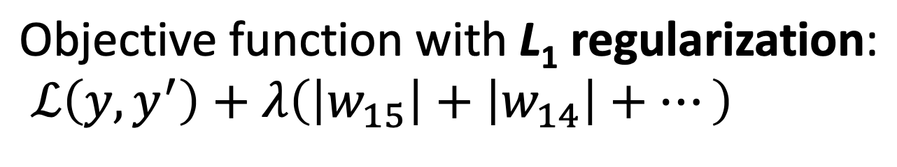
  • 1-norm, first-norm을 additional term으로 사용한다.
  • parameters/final solution이 sparse해진다.

✔️ L2를 사용하냐, L1을 사용하냐에 따라 optimization을 통해 얻은 parameter의 값이 살짝 달라지기 때문에, 어떤 종류의 solution을 얻고 싶은지에 따라 다른 type의 regularization을 사용해야 한다.

Popular Classifier

• Logistic Regression

• Support Vector Machine

  • 두 class 사이의 margin을 maximaze함으로써 model이 generalization performance를 달성하도록 도와준다.
  • constrained optimization(using KKT theorem) or gradient descent with hinge loss를 통해 train한다.

• Decision Tree

• Emsembles

  • 성능을 향상시키기 위해 multiple classifier(low capacity, simple easy function, low power function)을 사용한다.

  • Type

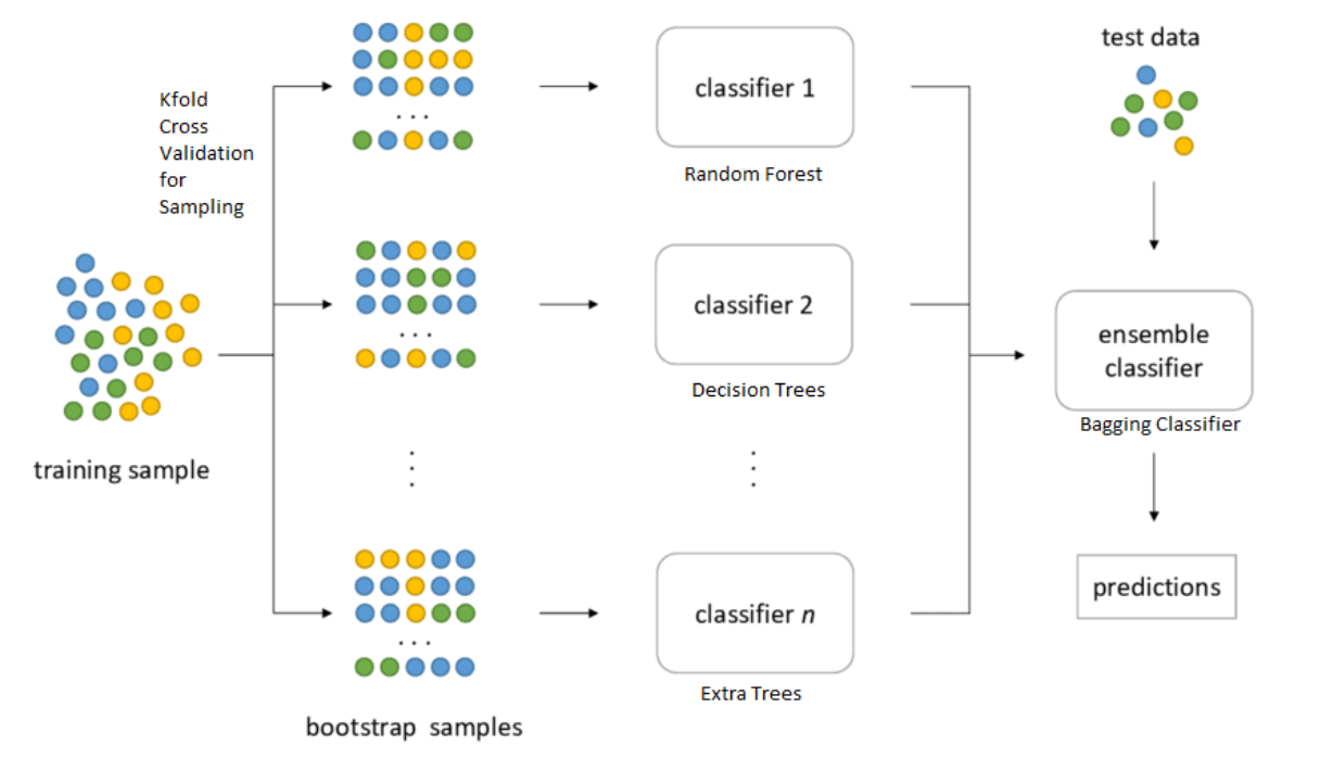
    • Bagging : different subsets of data 혹은 different subsets of features에 대해 multiple classifier를 훈련한다. classifier들이 same level에 있다.
      

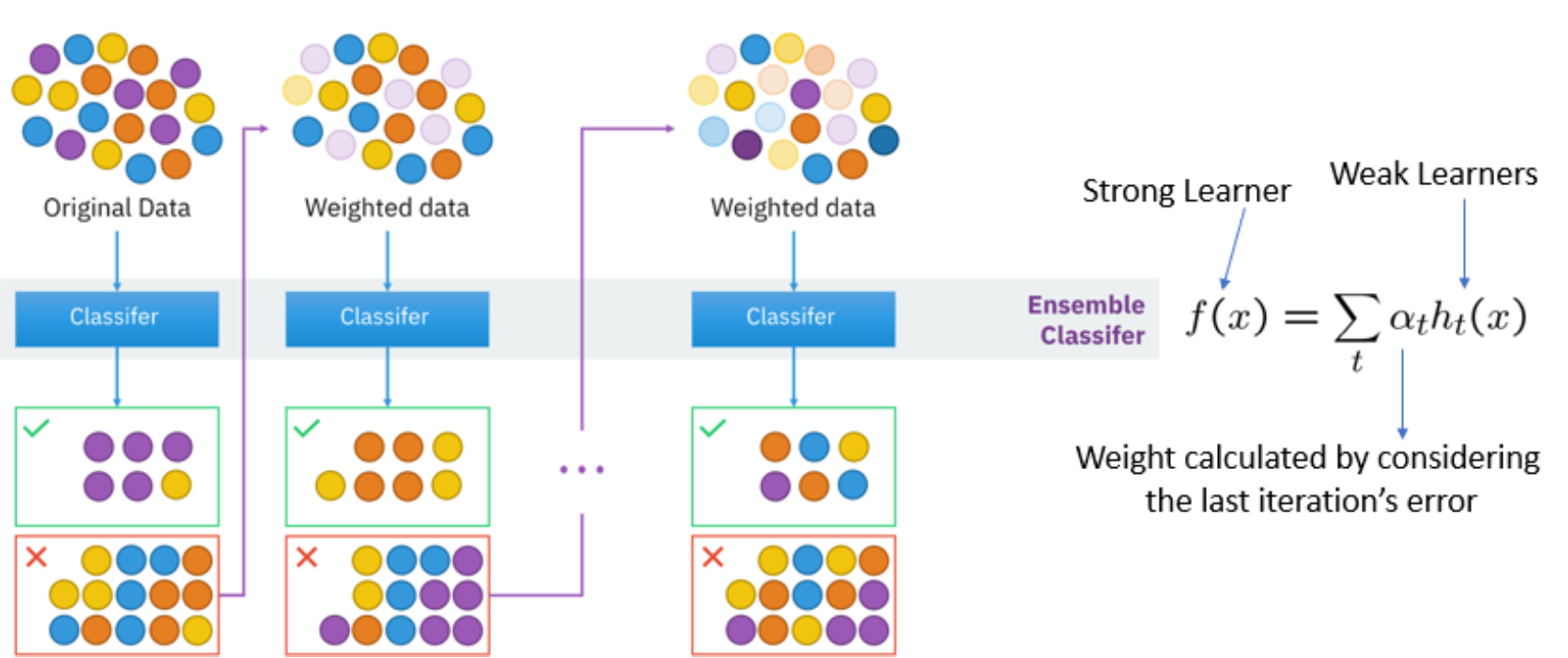
    • Boosting : classifier가 hierarchical적인 특징을 갖는다. weak learners, series of weak functions의 chain을 이용하여 문제를 조금씩 조금씩 해결한다. Wrong classify 한 것을 next level로 보내고 another function을 train하여 classification하고 wrong classify 한 것을 보내고 이것을 반복한다.
      

• K-means

  • hard clustering : 한 sample은 한번에 오직 한 cluster에만 속할 수 있다.
  • geometric

• Mixture of Gaussian (clustering)
  

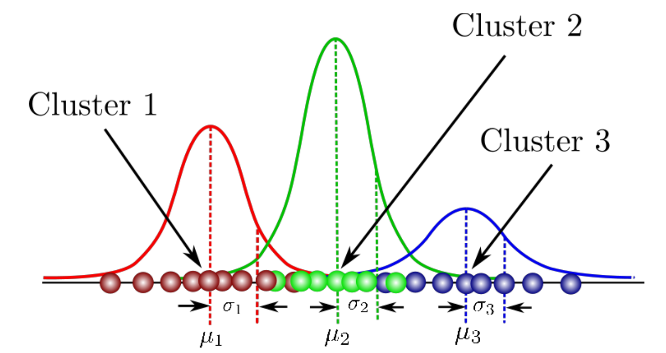
  • soft clustering
  • K-means를 probabilistic spin을 넣어 generalize한 것이다.
  • 각 cluster가 gaussian distribution이라고 가정한다.
  • sample이 probabilistically하게 각 cluster에 속한다. Ex. 이 sample이 cluster 1일 확률 30%, cluster 2일 확률 10%, cluster 3일 확률 거의 0%
  • Expectation-Maximization(EM)을 통해 훈련한다.

Reference

• AI504: Programming for AI Lecture at KAIST AI