Week 6: Generative adversarial network (GAN)
written by Jihoon-Tack (jihoontack@kaist.ac.kr)
modified by Sungjin-Park (zxznm@kaist.ac.kr)
- We will cover basic concepts of GAN & implement vanilla GAN [Goodfellow et al., NIPS 2014]
- We will give basic skeletone code which include (1) training structure (2) sample visualization (3) FID evaluation
- You should implement (1) generator & discriminator architecture (2) noise sampling (3) GAN loss
- Additionally, will give you DCGAN (basic GAN architecture) code that you can enjoy by your-self
If you have any questions, feel free to ask
0. Preliminary
0.1. Prelim step 1: Load packages & GPU setup
# visualize current GPU usages in your server
!nvidia-smi
Tue Mar 14 06:44:12 2023
+-----------------------------------------------------------------------------+
| NVIDIA-SMI 525.85.12 Driver Version: 525.85.12 CUDA Version: 12.0 |
|-------------------------------+----------------------+----------------------+
| GPU Name Persistence-M| Bus-Id Disp.A | Volatile Uncorr. ECC |
| Fan Temp Perf Pwr:Usage/Cap| Memory-Usage | GPU-Util Compute M. |
| | | MIG M. |
|===============================+======================+======================|
| 0 NVIDIA A100-SXM... Off | 00000000:00:04.0 Off | 0 |
| N/A 33C P0 51W / 400W | 0MiB / 40960MiB | 0% Default |
| | | Disabled |
+-------------------------------+----------------------+----------------------+
+-----------------------------------------------------------------------------+
| Processes: |
| GPU GI CI PID Type Process name GPU Memory |
| ID ID Usage |
|=============================================================================|
| No running processes found |
+-----------------------------------------------------------------------------+# set gpu by number
import os
import random
os.environ['CUDA_VISIBLE_DEVICES'] = '0' # setting gpu number# load packages
import numpy as np
import matplotlib.pyplot as plt
import matplotlib.animation as animation
import imageio #### install with "pip install imageio"
from IPython.display import HTML
import torch
import torch.nn as nn
import torch.nn.parallel
import torch.backends.cudnn as cudnn
import torch.optim as optim
import torch.utils.data
import torchvision.datasets as dset
import torchvision.transforms as transforms
import torchvision.utils as vutils
from torchvision.utils import make_grid# Create folders
if not os.path.exists('./checkpoint'):
os.mkdir('./checkpoint')
if not os.path.exists('./dataset'):
os.mkdir('./dataset')
if not os.path.exists('./img'):
os.mkdir('./img')
if not os.path.exists('./img/real'):
os.mkdir('./img/real')
if not os.path.exists('./img/fake'):
os.mkdir('./img/fake')0.2. Prelim step 2: Define visualization & image saving code
# visualize the first image from the torch tensor
def vis_image(image):
    plt.imshow(image[0].detach().cpu().numpy(),cmap='gray')
    plt.show()
def save_gif(training_progress_images, images):
'''
training_progress_images: list of training images generated each iteration
images: image that is generated in this iteration
'''
img_grid = make_grid(images.data)
img_grid = np.transpose(img_grid.detach().cpu().numpy(), (1, 2, 0))
img_grid = 255. * img_grid
img_grid = img_grid.astype(np.uint8)
training_progress_images.append(img_grid)
imageio.mimsave('./img/training_progress.gif', training_progress_images)
return training_progress_images# visualize gif file
def vis_gif(training_progress_images):
fig = plt.figure()
ims = []
for i in range(len(training_progress_images)):
im = plt.imshow(training_progress_images[i], animated=True)
ims.append([im])
ani = animation.ArtistAnimation(fig, ims, interval=50, blit=True, repeat_delay=1000)
html = ani.to_html5_video()
HTML(html)# visualize gif file
def plot_gif(training_progress_images, plot_length=10):
plt.close()
fig = plt.figure()
total_len = len(training_progress_images)
for i in range(plot_length):
im = plt.imshow(training_progress_images[int(total_len/plot_length)*i])
plt.show()def save_image_list(dataset, real):
if real:
base_path = './img/real'
else:
base_path = './img/fake'
dataset_path = []
for i in range(len(dataset)):
save_path = f'{base_path}/image_{i}.png'
dataset_path.append(save_path)
vutils.save_image(dataset[i], save_path)
return base_path0.3. Prelim step 3: Load dataset, define dataloader
In this class we will use MNIST (or you can use Fashion-MNIST) due to the time constraint :( \
You can practice with CIFAR-10 by your-self since dataset is already implemented inside PyTorch!
- Simply use
dataset=dset.CIFAR10(.)function in PyTorch. - If you are using CIFAR dataset, please note that the resolution is different to MNIST and should change model input dimension.
dataset = dset.MNIST(root="./dataset", download=True,
                                   transform=transforms.Compose([
                                   transforms.ToTensor(),
                ]))
# If you want to download FMNIST use dset.FashionMNIST
# dataset = dset.FashionMNIST(.)

dataloader = torch.utils.data.DataLoader(dataset, batch_size=128, shuffle=True, num_workers=2)
Downloading http://yann.lecun.com/exdb/mnist/train-images-idx3-ubyte.gz
Downloading http://yann.lecun.com/exdb/mnist/train-images-idx3-ubyte.gz to ./dataset/MNIST/raw/train-images-idx3-ubyte.gz
0%| | 0/9912422 [00:00<?, ?it/s]
Extracting ./dataset/MNIST/raw/train-images-idx3-ubyte.gz to ./dataset/MNIST/raw
Downloading http://yann.lecun.com/exdb/mnist/train-labels-idx1-ubyte.gz
Downloading http://yann.lecun.com/exdb/mnist/train-labels-idx1-ubyte.gz to ./dataset/MNIST/raw/train-labels-idx1-ubyte.gz
0%| | 0/28881 [00:00<?, ?it/s]
Extracting ./dataset/MNIST/raw/train-labels-idx1-ubyte.gz to ./dataset/MNIST/raw
Downloading http://yann.lecun.com/exdb/mnist/t10k-images-idx3-ubyte.gz
Downloading http://yann.lecun.com/exdb/mnist/t10k-images-idx3-ubyte.gz to ./dataset/MNIST/raw/t10k-images-idx3-ubyte.gz
0%| | 0/1648877 [00:00<?, ?it/s]
Extracting ./dataset/MNIST/raw/t10k-images-idx3-ubyte.gz to ./dataset/MNIST/raw
Downloading http://yann.lecun.com/exdb/mnist/t10k-labels-idx1-ubyte.gz
Downloading http://yann.lecun.com/exdb/mnist/t10k-labels-idx1-ubyte.gz to ./dataset/MNIST/raw/t10k-labels-idx1-ubyte.gz
0%| | 0/4542 [00:00<?, ?it/s]
Extracting ./dataset/MNIST/raw/t10k-labels-idx1-ubyte.gz to ./dataset/MNIST/raw1. Define your generator & discriminator
1.1. Define generator module
class Generator(nn.Module):
    def __init__(self):
        super(Generator, self).__init__()
        self.main = nn.Sequential(
            #########################
            # Define your own generator #
            #########################
            nn.Linear(100, 256),
            nn.ReLU(),
            nn.Linear(256, 256),
            nn.ReLU(),
            nn.Linear(256,784),
            nn.Sigmoid(), # 0-1
            #########################
        )

    def forward(self, input):
        #####################################
        # Change the shape of output if necessary #

        # input_shape = batch_size, 100
        #####################################

        output = self.main(input)

        #####################################
        # Change the shape of output if necessary #
        output = output.view(-1, 1, 28, 28)
        #####################################
        return output
1.2. Define discriminator module
class Discriminator(nn.Module):
    def __init__(self):
        super(Discriminator, self).__init__()
        self.main = nn.Sequential(

            ############################
            # Define your own discriminator #
            ############################
            nn.Linear(28*28, 256),
            nn.LeakyReLU(0.2),
            nn.Linear(256, 256),
            nn.LeakyReLU(0.2),
            nn.Linear(256,1),
            nn.Sigmoid(),
            ############################
        )

    def forward(self, input):
        #####################################
        # Change the shape of output if necessary #
        # Batch * 1 * 28 * 28
        input = input.view(-1, 28*28)
        #####################################

        output = self.main(input)

        #####################################
        # Change the shape of output if necessary # (batch_size, 1) -> (batch_size, )
        output = output.squeeze(dim=1)
        #####################################

        return output
1.3. Upload on GPU, define optimizer
netG = Generator().cuda()
netD = Discriminator().cuda()

optimizerD = optim.Adam(netD.parameters(), lr=0.0002)
optimizerG = optim.Adam(netG.parameters(), lr=0.0002)
2. Noise sampling
#### Implement here ####
#### Batch=128 * Dimension=100
noise = torch.randn(128,100).cuda() # sampling the value from normal distribution
3. Train GAN
Objective
Pseudo-code
Implement GAN by filling out the following blankes!
from numpy.ma.core import outerproduct
fixed_noise = torch.randn(128,100).cuda()

criterion = nn.BCELoss()

n_epoch = 200
training_progress_images_list = []
for epoch in range(n_epoch):
    for i, (data, _) in enumerate(dataloader):
        ####################################################
        # (1) Update D network: maximize log(D(x)) + log(1 - D(G(z))) #
        ###################################################
        # train with real
        netD.zero_grad()
        data = data.cuda()
        batch_size = data.size(0)

        label = torch.ones((batch_size,)).cuda() # real label = 1
        output = netD(data)
        errD_real = criterion(output, label)

        # train with fake
        noise = torch.randn(batch_size, 100).cuda()
        fake = netG(noise)
        label = torch.zeros((batch_size,)).cuda() # fake label
        output = netD(fake.detach()) # Detach from computational graph only for this line. Ensure that we do not update the generator network while we training discriminator network
        errD_fake = criterion(output, label)

        # Loss backward
        errD = errD_real + errD_fake
        errD.backward()
        optimizerD.step()

        ########################################
        # (2) Update G network: maximize log(D(G(z))) #
        ########################################
        netG.zero_grad()
        label = torch.ones((batch_size,)).cuda() # fake labels are real for generator cost
        output = netD(fake)
        errG = criterion(output, label)

        errG.backward()
        optimizerG.step()

    print('[%d/%d] Loss_D: %.4f Loss_G: %.4f'
              % (epoch, n_epoch, errD.item(), errG.item()))

    #save the output
    fake = netG(fixed_noise)
    training_progress_images_list = save_gif(training_progress_images_list, fake)  # Save fake image while training!

    # Check pointing for every epoch
    torch.save(netG.state_dict(), './checkpoint/netG_epoch_%d.pth' % (epoch))
    torch.save(netD.state_dict(), './checkpoint/netD_epoch_%d.pth' % (epoch))
[0/200] Loss_D: 0.0278 Loss_G: 5.2332
[1/200] Loss_D: 0.0067 Loss_G: 6.6924
[2/200] Loss_D: 0.0055 Loss_G: 7.0066
[3/200] Loss_D: 0.0232 Loss_G: 6.6146
[4/200] Loss_D: 0.0051 Loss_G: 6.9175
[5/200] Loss_D: 0.0097 Loss_G: 7.9294
[6/200] Loss_D: 0.0452 Loss_G: 7.0327
[7/200] Loss_D: 0.0087 Loss_G: 6.2442
[8/200] Loss_D: 0.0383 Loss_G: 7.3042
[9/200] Loss_D: 0.0168 Loss_G: 8.2150
[10/200] Loss_D: 0.0077 Loss_G: 7.3655
[11/200] Loss_D: 0.0051 Loss_G: 11.6685
[12/200] Loss_D: 0.0117 Loss_G: 7.4554
[13/200] Loss_D: 0.0332 Loss_G: 10.1345
[14/200] Loss_D: 0.0086 Loss_G: 7.9291
[15/200] Loss_D: 0.0198 Loss_G: 8.1875
[16/200] Loss_D: 0.0442 Loss_G: 8.5643
[17/200] Loss_D: 0.0251 Loss_G: 8.9957
[18/200] Loss_D: 0.0247 Loss_G: 8.7191
[19/200] Loss_D: 0.0993 Loss_G: 6.5718
[20/200] Loss_D: 0.0625 Loss_G: 6.9238
[21/200] Loss_D: 0.0876 Loss_G: 6.2759
[22/200] Loss_D: 0.0516 Loss_G: 7.8121
[23/200] Loss_D: 0.0473 Loss_G: 7.4642
[24/200] Loss_D: 0.0287 Loss_G: 7.8002
[25/200] Loss_D: 0.1131 Loss_G: 7.4242
[26/200] Loss_D: 0.0928 Loss_G: 7.7899
[27/200] Loss_D: 0.0611 Loss_G: 7.3804
[28/200] Loss_D: 0.1526 Loss_G: 6.9164
[29/200] Loss_D: 0.2670 Loss_G: 5.4927
[30/200] Loss_D: 0.1773 Loss_G: 6.4207
[31/200] Loss_D: 0.1986 Loss_G: 6.8739
[32/200] Loss_D: 0.0941 Loss_G: 5.5342
[33/200] Loss_D: 0.1266 Loss_G: 6.0398
[34/200] Loss_D: 0.1972 Loss_G: 6.3810
[35/200] Loss_D: 0.1186 Loss_G: 5.5829
[36/200] Loss_D: 0.1497 Loss_G: 4.8458
[37/200] Loss_D: 0.2537 Loss_G: 4.7663
[38/200] Loss_D: 0.3679 Loss_G: 5.0121
[39/200] Loss_D: 0.1673 Loss_G: 4.0175
[40/200] Loss_D: 0.1909 Loss_G: 3.7317
[41/200] Loss_D: 0.3479 Loss_G: 4.5463
[42/200] Loss_D: 0.2570 Loss_G: 3.8854
[43/200] Loss_D: 0.2342 Loss_G: 3.4809
[44/200] Loss_D: 0.3282 Loss_G: 3.9486
[45/200] Loss_D: 0.3666 Loss_G: 3.1167
[46/200] Loss_D: 0.3041 Loss_G: 3.4950
[47/200] Loss_D: 0.4229 Loss_G: 3.4868
[48/200] Loss_D: 0.3967 Loss_G: 2.7635
[49/200] Loss_D: 0.5303 Loss_G: 3.4349
[50/200] Loss_D: 0.4610 Loss_G: 3.3140
[51/200] Loss_D: 0.3000 Loss_G: 2.9463
[52/200] Loss_D: 0.4263 Loss_G: 3.0674
[53/200] Loss_D: 0.4945 Loss_G: 2.5285
[54/200] Loss_D: 0.6044 Loss_G: 2.6387
[55/200] Loss_D: 0.6398 Loss_G: 2.7374
[56/200] Loss_D: 0.4782 Loss_G: 2.7014
[57/200] Loss_D: 0.4081 Loss_G: 2.9006
[58/200] Loss_D: 0.6929 Loss_G: 2.3315
[59/200] Loss_D: 0.6493 Loss_G: 2.1811
[60/200] Loss_D: 0.5600 Loss_G: 3.1068
[61/200] Loss_D: 0.5370 Loss_G: 2.3473
[62/200] Loss_D: 0.6882 Loss_G: 2.4993
[63/200] Loss_D: 0.6307 Loss_G: 2.8488
[64/200] Loss_D: 0.4929 Loss_G: 2.4295
[65/200] Loss_D: 0.6688 Loss_G: 2.1748
[66/200] Loss_D: 0.6310 Loss_G: 2.0889
[67/200] Loss_D: 0.6702 Loss_G: 2.2712
[68/200] Loss_D: 0.6278 Loss_G: 1.9477
[69/200] Loss_D: 0.5559 Loss_G: 2.6135
[70/200] Loss_D: 0.6944 Loss_G: 2.0490
[71/200] Loss_D: 0.6765 Loss_G: 2.3412
[72/200] Loss_D: 0.5467 Loss_G: 2.0005
[73/200] Loss_D: 0.4552 Loss_G: 2.5143
[74/200] Loss_D: 0.5896 Loss_G: 2.6358
[75/200] Loss_D: 0.5136 Loss_G: 2.1075
[76/200] Loss_D: 0.6540 Loss_G: 1.8072
[77/200] Loss_D: 0.5514 Loss_G: 1.9645
[78/200] Loss_D: 0.6631 Loss_G: 2.1117
[79/200] Loss_D: 0.5816 Loss_G: 2.0202
[80/200] Loss_D: 0.6415 Loss_G: 2.1229
[81/200] Loss_D: 0.5997 Loss_G: 2.0477
[82/200] Loss_D: 0.6831 Loss_G: 2.1549
[83/200] Loss_D: 0.7160 Loss_G: 1.9122
[84/200] Loss_D: 0.6751 Loss_G: 2.1955
[85/200] Loss_D: 0.6912 Loss_G: 1.9617
[86/200] Loss_D: 0.6345 Loss_G: 1.6794
[87/200] Loss_D: 0.5733 Loss_G: 2.0072
[88/200] Loss_D: 0.6757 Loss_G: 1.7712
[89/200] Loss_D: 0.6003 Loss_G: 2.1516
[90/200] Loss_D: 0.6802 Loss_G: 1.9625
[91/200] Loss_D: 0.8673 Loss_G: 2.0585
[92/200] Loss_D: 0.5723 Loss_G: 2.0141
[93/200] Loss_D: 0.7011 Loss_G: 2.1104
[94/200] Loss_D: 0.6148 Loss_G: 2.0358
[95/200] Loss_D: 0.7255 Loss_G: 1.8161
[96/200] Loss_D: 0.6873 Loss_G: 1.7459
[97/200] Loss_D: 0.6397 Loss_G: 2.2145
[98/200] Loss_D: 0.6312 Loss_G: 1.9318
[99/200] Loss_D: 0.6197 Loss_G: 1.9805
[100/200] Loss_D: 0.6028 Loss_G: 1.9042
[101/200] Loss_D: 0.5530 Loss_G: 1.9147
[102/200] Loss_D: 0.5594 Loss_G: 2.0622
[103/200] Loss_D: 0.5754 Loss_G: 2.1670
[104/200] Loss_D: 0.6111 Loss_G: 1.8540
[105/200] Loss_D: 0.6443 Loss_G: 1.9582
[106/200] Loss_D: 0.7698 Loss_G: 1.7884
[107/200] Loss_D: 0.7679 Loss_G: 1.8875
[108/200] Loss_D: 0.6570 Loss_G: 2.1502
[109/200] Loss_D: 0.7878 Loss_G: 2.0280
[110/200] Loss_D: 0.7351 Loss_G: 1.8335
[111/200] Loss_D: 0.6549 Loss_G: 2.0732
[112/200] Loss_D: 0.6392 Loss_G: 1.9383
[113/200] Loss_D: 0.5362 Loss_G: 2.0843
[114/200] Loss_D: 0.6263 Loss_G: 1.8788
[115/200] Loss_D: 0.7242 Loss_G: 1.8431
[116/200] Loss_D: 0.6793 Loss_G: 1.7545
[117/200] Loss_D: 0.6305 Loss_G: 1.9253
[118/200] Loss_D: 0.7641 Loss_G: 1.7972
[119/200] Loss_D: 0.7153 Loss_G: 1.9617
[120/200] Loss_D: 0.7097 Loss_G: 1.7837
[121/200] Loss_D: 0.5486 Loss_G: 1.9558
[122/200] Loss_D: 0.6110 Loss_G: 1.9338
[123/200] Loss_D: 0.6684 Loss_G: 1.7228
[124/200] Loss_D: 0.8127 Loss_G: 1.5648
[125/200] Loss_D: 0.6146 Loss_G: 2.0209
[126/200] Loss_D: 0.6214 Loss_G: 1.8229
[127/200] Loss_D: 0.6086 Loss_G: 1.6487
[128/200] Loss_D: 0.6354 Loss_G: 2.0144
[129/200] Loss_D: 0.6393 Loss_G: 1.7239
[130/200] Loss_D: 0.7100 Loss_G: 1.8804
[131/200] Loss_D: 0.6952 Loss_G: 1.7529
[132/200] Loss_D: 0.6362 Loss_G: 1.9861
[133/200] Loss_D: 0.7402 Loss_G: 1.8417
[134/200] Loss_D: 0.5830 Loss_G: 1.9368
[135/200] Loss_D: 0.6995 Loss_G: 1.7797
[136/200] Loss_D: 0.4987 Loss_G: 2.3894
[137/200] Loss_D: 0.7826 Loss_G: 1.9992
[138/200] Loss_D: 0.7493 Loss_G: 2.0289
[139/200] Loss_D: 0.6406 Loss_G: 1.6912
[140/200] Loss_D: 0.7231 Loss_G: 2.0148
[141/200] Loss_D: 0.5875 Loss_G: 2.0120
[142/200] Loss_D: 0.7361 Loss_G: 2.2748
[143/200] Loss_D: 0.6991 Loss_G: 1.7514
[144/200] Loss_D: 0.7755 Loss_G: 2.0528
[145/200] Loss_D: 0.7739 Loss_G: 1.8485
[146/200] Loss_D: 0.5782 Loss_G: 2.0858
[147/200] Loss_D: 0.6258 Loss_G: 1.8898
[148/200] Loss_D: 0.5865 Loss_G: 1.9529
[149/200] Loss_D: 0.5956 Loss_G: 2.1187
[150/200] Loss_D: 0.5355 Loss_G: 2.1727
[151/200] Loss_D: 0.7037 Loss_G: 2.5136
[152/200] Loss_D: 0.7161 Loss_G: 2.0995
[153/200] Loss_D: 0.7428 Loss_G: 1.6995
[154/200] Loss_D: 0.6751 Loss_G: 2.0279
[155/200] Loss_D: 0.6100 Loss_G: 2.0065
[156/200] Loss_D: 0.6219 Loss_G: 1.7515
[157/200] Loss_D: 0.6225 Loss_G: 1.7392
[158/200] Loss_D: 0.6902 Loss_G: 1.6894
[159/200] Loss_D: 0.4571 Loss_G: 2.3035
[160/200] Loss_D: 0.6984 Loss_G: 1.9174
[161/200] Loss_D: 0.5690 Loss_G: 2.0046
[162/200] Loss_D: 0.7983 Loss_G: 1.7482
[163/200] Loss_D: 0.7642 Loss_G: 1.6775
[164/200] Loss_D: 0.7108 Loss_G: 1.9362
[165/200] Loss_D: 0.7017 Loss_G: 2.0730
[166/200] Loss_D: 0.5509 Loss_G: 1.7979
[167/200] Loss_D: 0.7129 Loss_G: 2.1274
[168/200] Loss_D: 0.8619 Loss_G: 1.4474
[169/200] Loss_D: 0.6315 Loss_G: 1.8887
[170/200] Loss_D: 0.6720 Loss_G: 1.7378
[171/200] Loss_D: 0.5204 Loss_G: 2.0127
[172/200] Loss_D: 0.7019 Loss_G: 1.7550
[173/200] Loss_D: 0.6297 Loss_G: 1.9554
[174/200] Loss_D: 0.7956 Loss_G: 1.4933
[175/200] Loss_D: 0.5747 Loss_G: 1.8440
[176/200] Loss_D: 0.7734 Loss_G: 1.9882
[177/200] Loss_D: 0.5068 Loss_G: 2.1219
[178/200] Loss_D: 0.7795 Loss_G: 2.1137
[179/200] Loss_D: 0.8261 Loss_G: 1.7356
[180/200] Loss_D: 0.7234 Loss_G: 1.9543
[181/200] Loss_D: 0.7960 Loss_G: 1.7290
[182/200] Loss_D: 0.5939 Loss_G: 1.7928
[183/200] Loss_D: 0.6671 Loss_G: 1.8297
[184/200] Loss_D: 0.5158 Loss_G: 2.0038
[185/200] Loss_D: 0.5259 Loss_G: 1.9971
[186/200] Loss_D: 0.5076 Loss_G: 1.9064
[187/200] Loss_D: 0.5963 Loss_G: 2.2020
[188/200] Loss_D: 0.5936 Loss_G: 2.1423
[189/200] Loss_D: 0.5988 Loss_G: 1.8684
[190/200] Loss_D: 0.7734 Loss_G: 1.8150
[191/200] Loss_D: 0.6033 Loss_G: 1.8027
[192/200] Loss_D: 0.8170 Loss_G: 2.0003
[193/200] Loss_D: 0.8149 Loss_G: 2.0378
[194/200] Loss_D: 0.6591 Loss_G: 2.1802
[195/200] Loss_D: 0.7129 Loss_G: 1.6738
[196/200] Loss_D: 0.7404 Loss_G: 1.8643
[197/200] Loss_D: 0.8608 Loss_G: 1.6103
[198/200] Loss_D: 0.6511 Loss_G: 1.7139
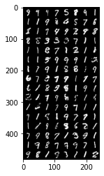
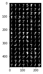
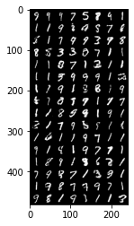
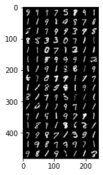
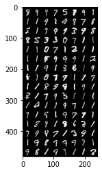
[199/200] Loss_D: 0.5681 Loss_G: 1.97744. Visualize/Plot your generated samples
plot_gif(training_progress_images_list)
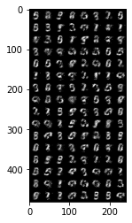
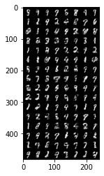
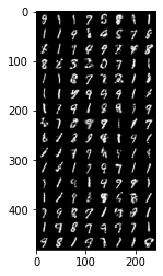
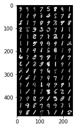
5. Evaluate your model: Fréchet Inception Distance (FID) score
How to evaluate the equality of your generated sample?\
Maybe training loss...? No!
Papers have shown that training loss might not be the best metric!
There are many evaluation metric that has been proposed and most famous metric is as follows: Inception score, Fréchet Inception Distance
In this course, we will handle Fréchet Inception Distance (FID) score.
5.1. What is FID score?
FID measures the distance between real dataset & fake dataset in feature space of Inception pretrained network.\
From the extracted features of real & fake dataset, we can compute mean & covariance of each features to calculate the distance between distributions.
For the implementation, we simply use the source code from github: https://github.com/mseitzer/pytorch-fid
Please note that Inception network is pretrained on ImageNet, therefore the MNIST FID score might be unrealiable.\
5.2. Load FID score function: code is from the github
import inception
import fid_score
from fid_score import calculate_fid_given_paths
5.3. Evaluate your model (save samples!!)
The Inception network's input resolution is 224 by 224, we upscale small resolution datasets (e.g., MNSIT, CIFAR) into same resolution.
Please note that, we only save 50 samples in this lecture, however in practice we use full test dataset: reference
test_dataset = dset.MNIST(root="./dataset", download=True, train=False,
                                           transform=transforms.Compose([
                                           transforms.ToTensor(),
                        ]))

dataloader = torch.utils.data.DataLoader(test_dataset, batch_size=50, shuffle=True, num_workers=2)

for i, (data, _) in enumerate(dataloader):
    real_dataset = data
    break

noise = torch.randn(50, 100).cuda()
fake_dataset = netG(noise)
real_image_path_list = save_image_list(real_dataset, True)
fake_image_path_list = save_image_list(fake_dataset, False)5.4 Evaluate FID score
# calculate_fid_given_paths(paths, batch_size, cuda, dims)
fid_value = calculate_fid_given_paths([real_image_path_list, fake_image_path_list],
                                                          50,
                                                          True,
                                                          2048)
/usr/local/lib/python3.9/dist-packages/torchvision/models/_utils.py:208: UserWarning: The parameter 'pretrained' is deprecated since 0.13 and may be removed in the future, please use 'weights' instead.
warnings.warn(
/usr/local/lib/python3.9/dist-packages/torchvision/models/_utils.py:223: UserWarning: Arguments other than a weight enum or `None` for 'weights' are deprecated since 0.13 and may be removed in the future. The current behavior is equivalent to passing `weights=None`.
warnings.warn(msg)
Downloading: "https://github.com/mseitzer/pytorch-fid/releases/download/fid_weights/pt_inception-2015-12-05-6726825d.pth" to /root/.cache/torch/hub/checkpoints/pt_inception-2015-12-05-6726825d.pth
0%| | 0.00/91.2M [00:00<?, ?B/s]
100%|██████████| 1/1 [00:03<00:00, 3.86s/it]
100%|██████████| 1/1 [00:00<00:00, 24.36it/s]print (f'FID score: {fid_value}')FID score: 104.05031612983979Additional: DCGAN (try it by your-self)
There are various modern architectures of GAN e.g., DCGAN, SNGAN, and also training methods e.g., WGAN, gradient penulty
You can try the following architecture to improve the quality of generation!
- Note that this version is for 64 by 64 resolution
nc = 3 # number of channels, RGB
nz = 100 # input noise dimension
ngf = 64 # number of generator filters
ndf = 64 #number of discriminator filters

class Generator(nn.Module):
    def __init__(self):
        super(Generator, self).__init__()
        self.main = nn.Sequential(
            # input is Z, going into a convolution
            nn.ConvTranspose2d(nz, ngf * 8, 4, 1, 0, bias=False),
            nn.BatchNorm2d(ngf * 8),
            nn.ReLU(True),
            # state size. (ngf*8) x 4 x 4
            nn.ConvTranspose2d(ngf * 8, ngf * 4, 4, 2, 1, bias=False),
            nn.BatchNorm2d(ngf * 4),
            nn.ReLU(True),
            # state size. (ngf*4) x 8 x 8
            nn.ConvTranspose2d(ngf * 4, ngf * 2, 4, 2, 1, bias=False),
            nn.BatchNorm2d(ngf * 2),
            nn.ReLU(True),
            # state size. (ngf*2) x 16 x 16
            nn.ConvTranspose2d(ngf * 2, ngf, 4, 2, 1, bias=False),
            nn.BatchNorm2d(ngf),
            nn.ReLU(True),
            # state size. (ngf) x 32 x 32
            nn.ConvTranspose2d(ngf, nc, 4, 2, 1, bias=False),
            nn.Tanh()
            # state size. (nc) x 64 x 64
        )

    def forward(self, input):
        output = self.main(input)
        return output
class Discriminator(nn.Module):
def __init__(self):
super(Discriminator, self).__init__()
self.main = nn.Sequential(
# input is (nc) x 64 x 64
nn.Conv2d(nc, ndf, 4, 2, 1, bias=False),
nn.LeakyReLU(0.2, inplace=True),
# state size. (ndf) x 32 x 32
nn.Conv2d(ndf, ndf * 2, 4, 2, 1, bias=False),
nn.BatchNorm2d(ndf * 2),
nn.LeakyReLU(0.2, inplace=True),
# state size. (ndf*2) x 16 x 16
nn.Conv2d(ndf * 2, ndf * 4, 4, 2, 1, bias=False),
nn.BatchNorm2d(ndf * 4),
nn.LeakyReLU(0.2, inplace=True),
# state size. (ndf*4) x 8 x 8
nn.Conv2d(ndf * 4, ndf * 8, 4, 2, 1, bias=False),
nn.BatchNorm2d(ndf * 8),
nn.LeakyReLU(0.2, inplace=True),
# state size. (ndf*8) x 4 x 4
nn.Conv2d(ndf * 8, 1, 4, 1, 0, bias=False),
nn.Sigmoid()
)
def forward(self, input):
output = self.main(input)
return output.view(-1, 1).squeeze(1)Reference
PyTorch official DCGAN tutorial: https://pytorch.org/tutorials/beginner/dcgan_faces_tutorial.html \
github 1: https://github.com/Ksuryateja/DCGAN-CIFAR10-pytorch/blob/master/gan_cifar.py \
github 2: https://github.com/mseitzer/pytorch-fid \
FID score: https://github.com/mseitzer/pytorch-fid \
Inception score: https://github.com/sbarratt/inception-score-pytorch
Reference
- AI504: Programming for AI Lecture at KAIST AI