Named Entity Recognition (NER)
🔗 Goal
- piece of text들을 훑어보고 person, locations, products, dates, times와 같은 entity category에 속한 word를 labeling, 분류한다.
🔗 How to do NER
- NER task를 하기 위해서는 context를 사용해야 한다.
Simple NER: Window classification using binary logistic classifier
💡 Idea
neighboring words의 context window에서 각 word를 classify
🔗Algorithm
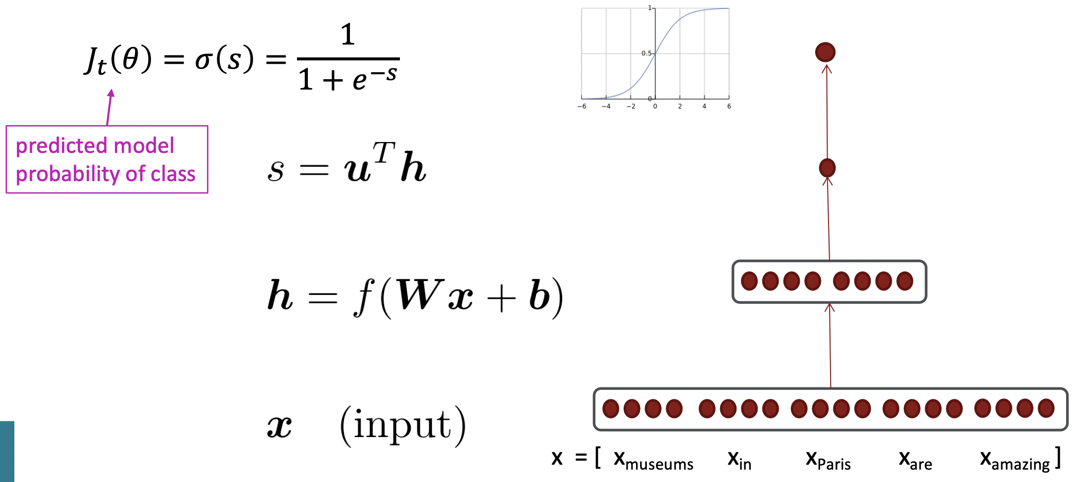
- "Paris"에 대해 window를 생성한다. 이 5개의 word에 대해 word2vec이나 GloVe word vectors를 사용해서 word vector를 얻은 다음, 5개의 vector를 concatenate하여 long vector를 만든다.
- D차원 word vector가 5개 있으므로 5D vector이다.
- 이 vector를 neural network의 layer에 넣는다. 이 layer는 vector를 matrix와 곱하고 bias vector를 추가한 다음, softmax transmation같은 non-linearity를 추가한다. 이렇게 하면 더 작은 차원을 가진 hidden vector가 나온다.
- extra vector u와 dot product하여 single real number를 얻는다.
- 마지막으로 이 single real number를 logistic transform에 넣어 word가 특정 class에 속할 확률을 예측한다.
❓ SGD를 계산하려면 loss function의 gradient를 계산해야 한다. 어떻게 계산할까?
1️⃣ Matrix calculas(computing gradients by hand)
Jacobian Matrix
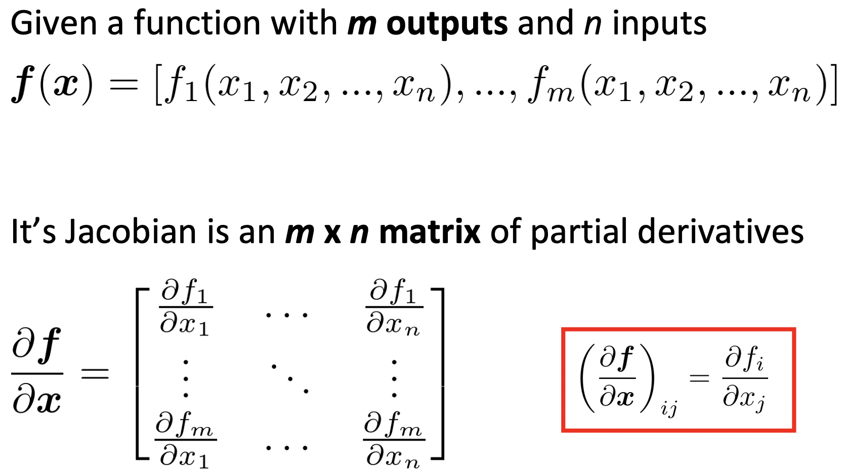
- 모든 가능한 input variable에 대한 output variable의 편미분을 가진다.
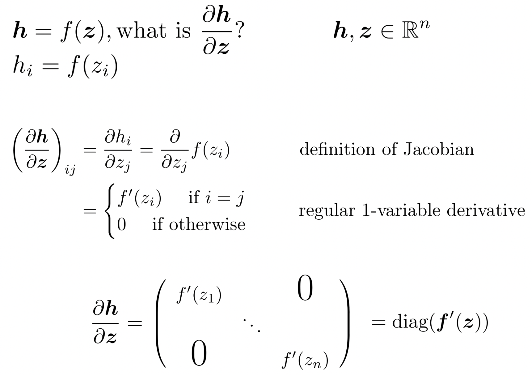
✔️ Example Jacobian: Elementwise activation Function
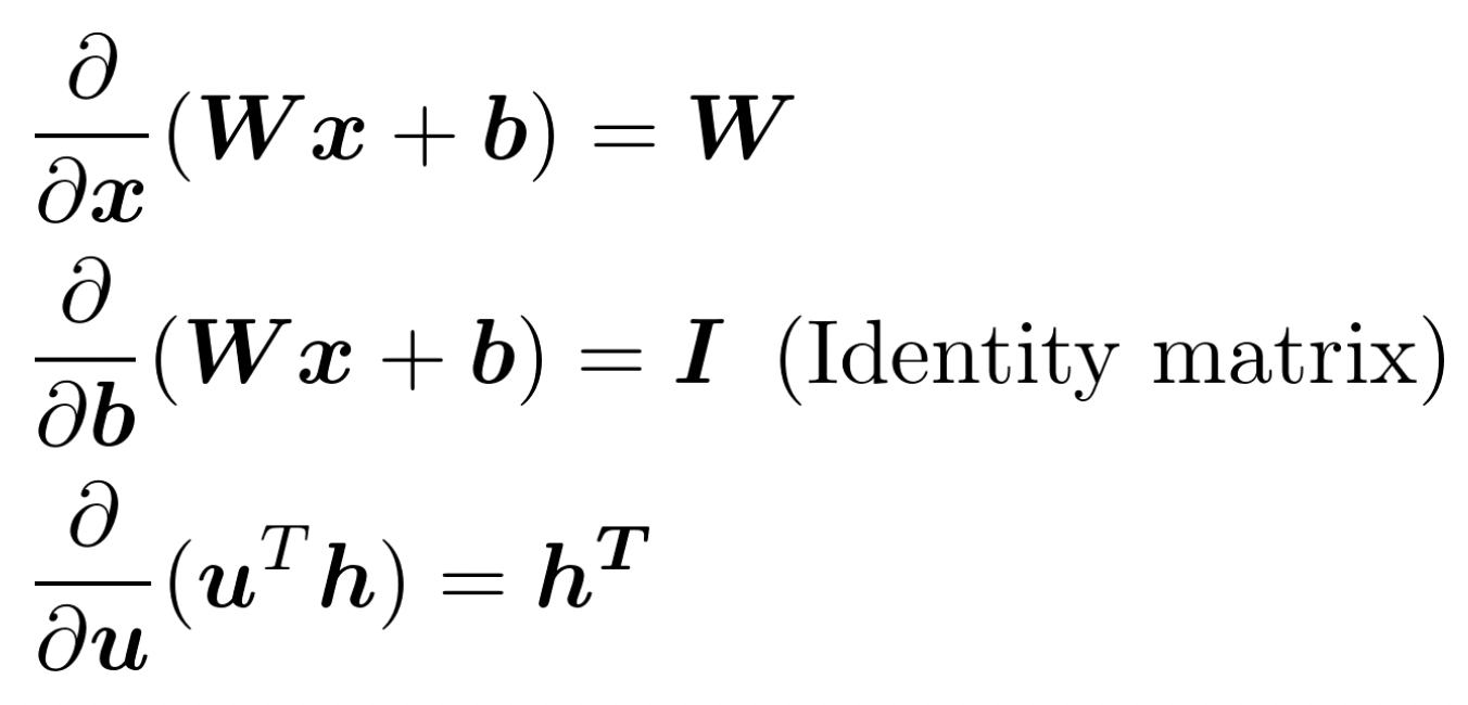
✔️ Other Jacobians
Chain Rule
- 한 변수에 대한 함수로 이루어져 있을 때 : multiply derivatives
- 다변수에 대한 함수로 이루어져 있을 때 : multiply Jacobians
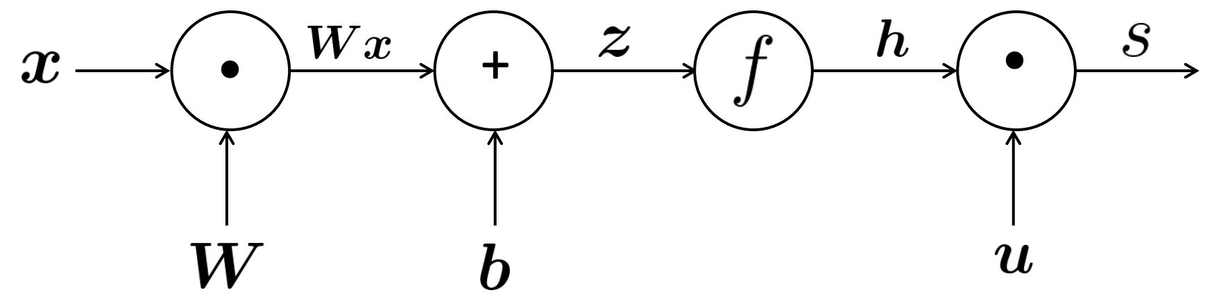
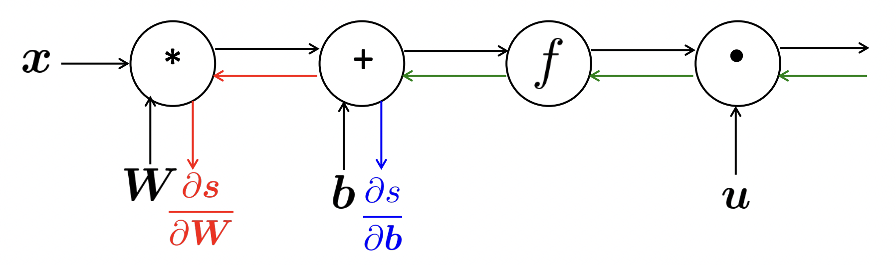
Window classification에서의 gradient update 과정
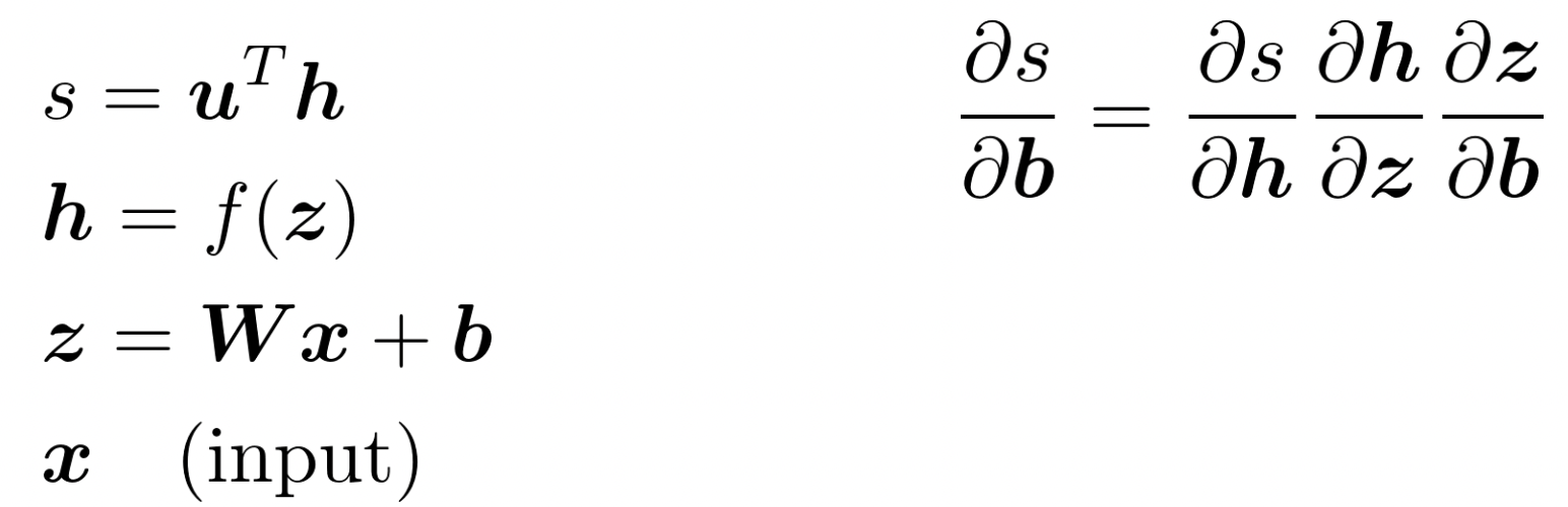
🔗 먼저 gradient of s with respect to b를 계산해보자.
1. Break up equations into simple pieces
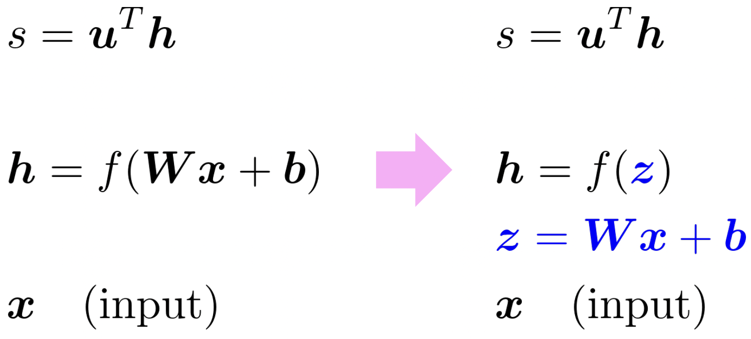
- variable들이 무엇인지 확실히 파악한다.
- 각 variable의 dimension이 무엇인지 보고, 결과의 dimension을 확인함으로써 내 계산을 검증한다.
2. Apply the chain rule
3. Write out the Jacobians
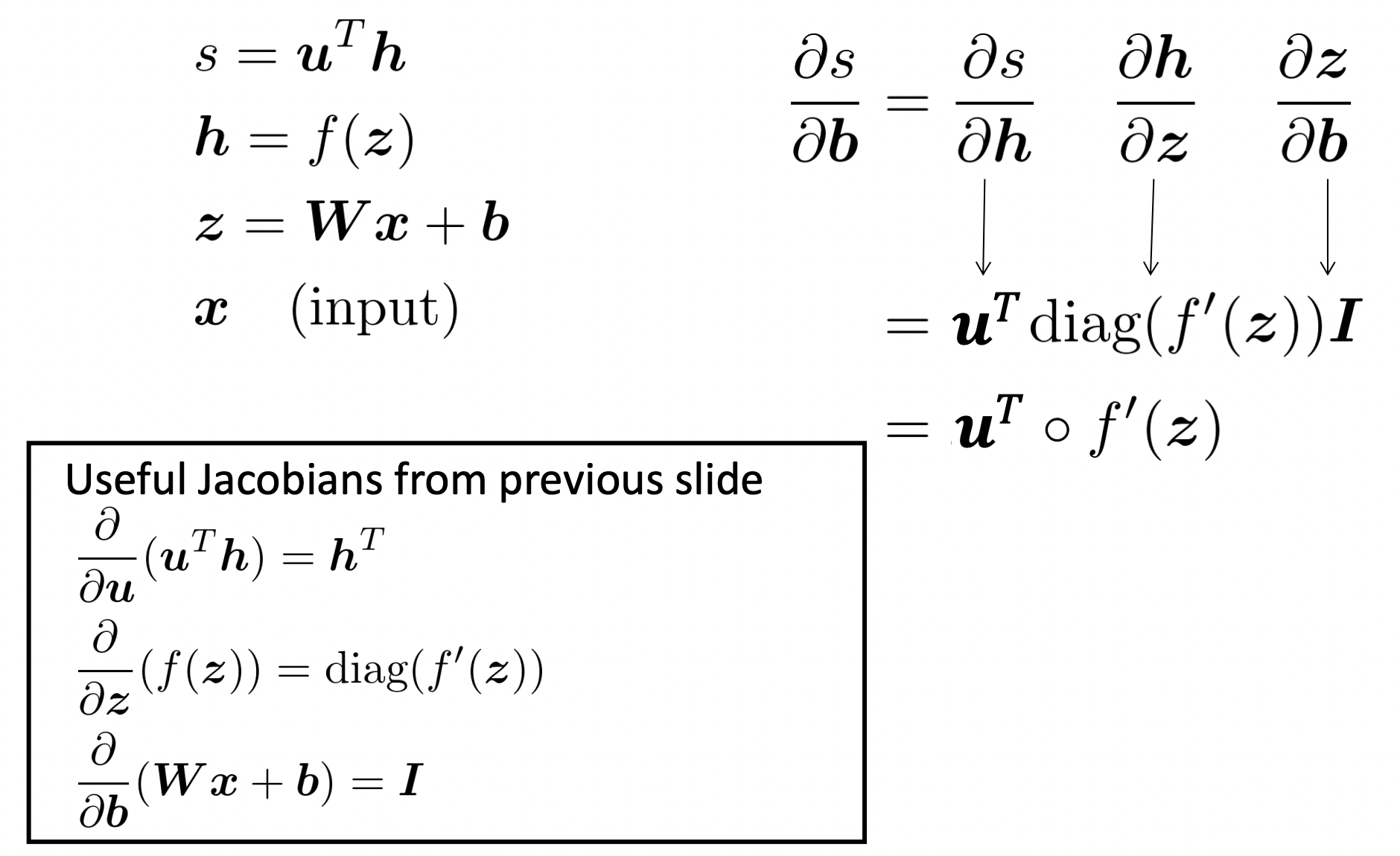
👉 Hadamard product : vector와 diagonal matrix를 곱할 때 쓸 수 있다.
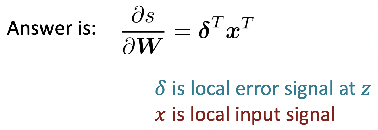
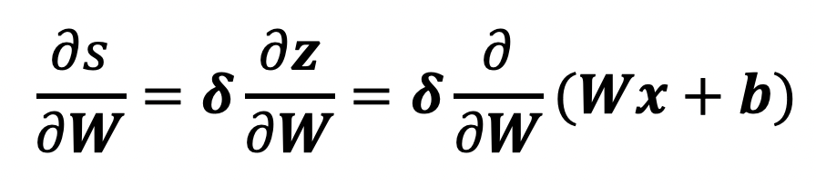
🔗 이제 gradient of s with respect to W를 계산해보자.
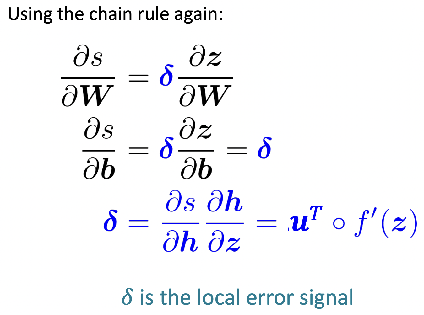
- 문제 : neural network를 효율적으로 train하기 위해서 반복되는 계산을 피하는 알고리즘을 사용하는 것이 필수적이다.
- 💡 해결 : 위에서 계산 되어진 편미분 값을 linear transform에 feed downward한다. feed downward된 값을 𝛅로 define한다.
- 𝛅 : local error signal
Shape convention
🔗 등장 배경
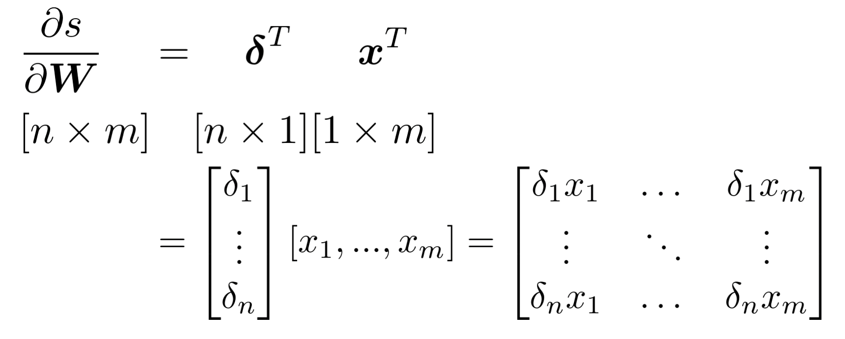
gradient of s with respect to W 의 Jacobian matrix를 구해보자.
W는 n*m matrix이고 s는 scaler value이다.
즉, output은 1개이고 Input은 n*m개이므로 Jacobian matrix는 1*n*m이 될 것이다.
하지만 SGD를 하려면 W가 n*m matrix이기 때문에 gradient도 W matrix와 동일한 shape이어야 -를 할 수 있다.
🔗 핵심
Jacobian을 reshape하여 원하는 matrix shape으로 바꾼다.
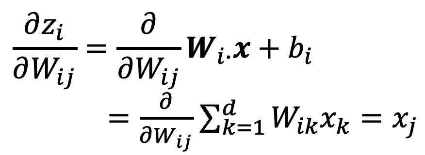
✔️Deriving local input gradient in backprop
- single weight 에 대해 생각하면 는 에만 기여한다.
✔️ Transposes를 통해 원하는 dimension을 만든다. outer product를 한다.
✔️ Shape convention에 대한 또 다른 예
- 위에서 계산한 gradient of s with respect to b 는 row vector이다. 하지만 b는 column vector이기 때문에 gradient도 column vector여야 한다. 따라서 transpose를 취해준다.
✔️ Disagreement between Jacobian form and the shape convention
1. Jacobian form은 chain rule을 쉽게 해주고 계산할 때 유용하므로 써야한다.
2. SGD를 하고 싶으면, gradient를 빼야하므로 shape convention을 통해 같은 shape을 가지도록 한다.
🔗 Two options
1. Jacobian form을 사용해서 모든 math를 풀고, 마지막에 shape convention을 따라 reshape하여 answer를 낸다.
- gradient of s with respect to b 를 계산할 때 했던 방식
- 항상 shape convention을 따른다.
- 어떤 shape이 나와야 하는지 dimension을 보고, transpose나 reshae를 한다. Jacobian form을 fully use하지 않는다.
- Hint : gradient는 항상 parameter와 shape이 같아야 한다. The error message 𝛅 that arrives at a hidden layer has the same dimensionality as that hidden layer. 이렇게 해서 항상 shape convention을 따르게 할 수 있다.
Backpropagation
- Backpropagation algorithm은 (generalized, multivariate, or matrix) chain rule을 사용하여 신중하게 derivative를 취하고 propagate 한다.
- Neural network는 shared structure와 shared derivatives가 많다. 그래서 higher layer에서 계산된 derivatives를 lower layers에서 derivatives를 계산할 때maximally, efficiently하게 re-use하여 연산량을 minimize한다.
Computational Graph
- Computational system에서 backpropagation을 하기 위해 computation graphs를 만든다.
- Source nodes: inputs
- Interior nodes: operations
- Edges : operation의 결과가 전달된다.
✔️ Forward Propagation
- input들을 가지고 output값을 계산한다.
✔️ Backpropagation
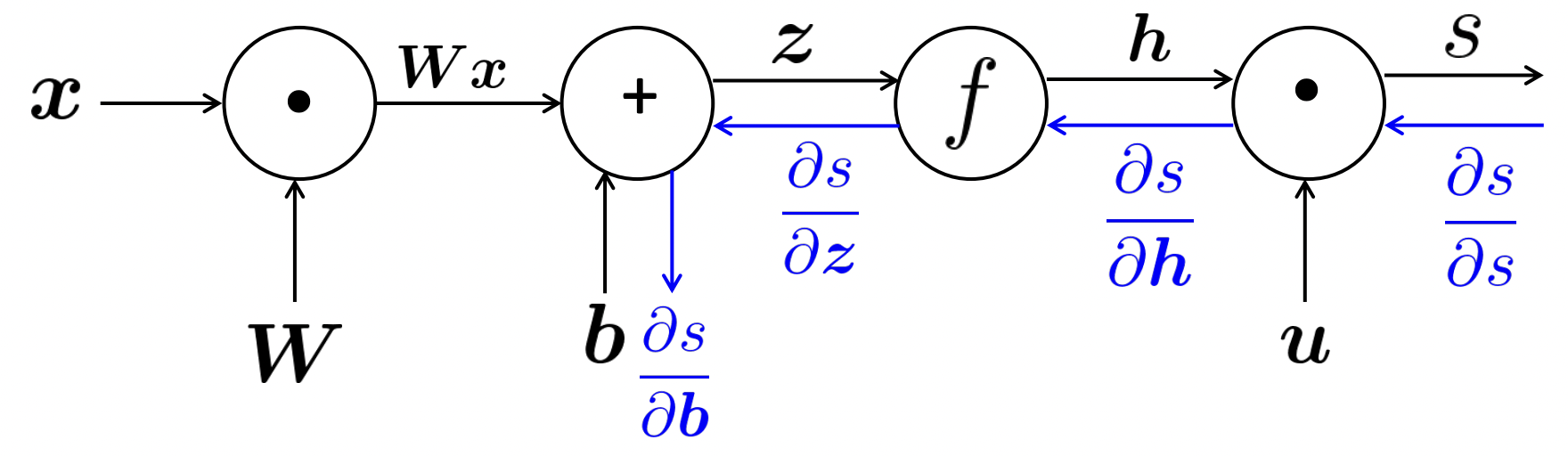
- Gradients를 edge의 반대방향으로 전달하여 model의 parameter를 어떻게 update해야 하는지 알려준다.
Backpropagation: Single Node
✔️ One output, one input
h = f(z)
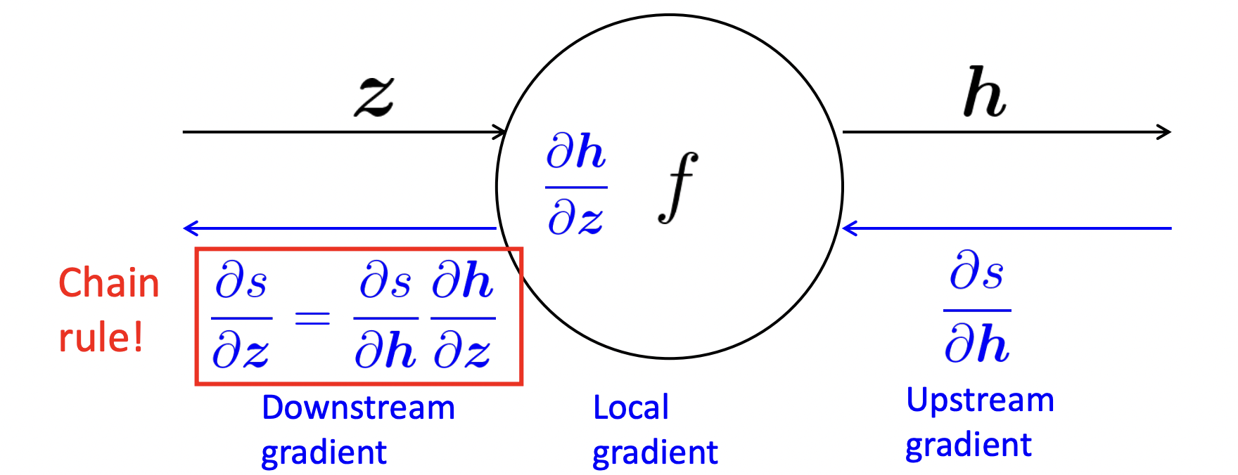
- 노드가 받게되는 것 : upstream gradient
- Goal : downstream gradient를 계산하여 넘겨준다.
- Local gradient : 각 노드가 가지고 있는 것으로, gradient of its output with respect to its input이다.
⭐️ General Principle
downstream gradient = upstream gradient * local gradient
✔️ One output, multiple input ➡️ multiple local gradients

- 노드가 받게 되는 것 : upstream gradient
- Goal : 각 input에 대한 local gradient를 구해서 각 local gradient에 대해서 chain rule을 사용해서 downstream gradient를 계산해 각각 넘겨준다.
An Example
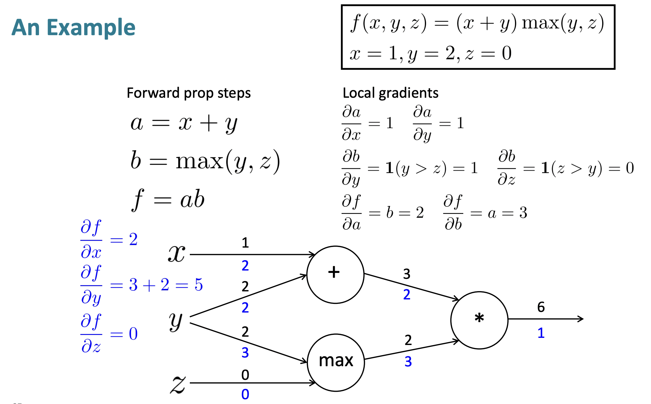
- Forward propagation
- Backpropagation
- 각 node에서의 local gradient를 모두 구하기
- Run backpropagation using chain rule
✔️ Multiple outward branches
- 받은 upstream gradient를 더한다.
Node Intuitions
- Addition : upstream gradient를 아래 있는 노드 각각에 "distributes"한다.
- Max : "routing" node같다. upstream gradient가 아래에 있는 branch들 중 하나에 다 가고 나머지들은 gradient가 없다.
- Multiplication : upstream gradient를 "swithces"하는 효과가 있다.
Efficiency
- 모든 gradient들을 한번만 계산한다.
- duplicated computation을 피하고 싶다.
- 초록색 gradient는 한 번만 계산한다.
Back-Prop in General Computation Graph
- 아무 parameter, input에도 의존하지 않는 starting point에서 시작한다.
- Compute forward propagation 시작한다.
- 현재 parameters 값과 현재 inputs 값을 이용하여 scalar값인 output z를 계산한다.
- directed graph에서 dependencies에 기반하여 topological sort order로 node를 방문한다.
- Run back propagation
- initialize output gradient = 1
- topological sort의 반대 순서로 node를 방분한다.
- successor에 대한 gradient를 사용하여 각 노드의 gradient를 계산한다.
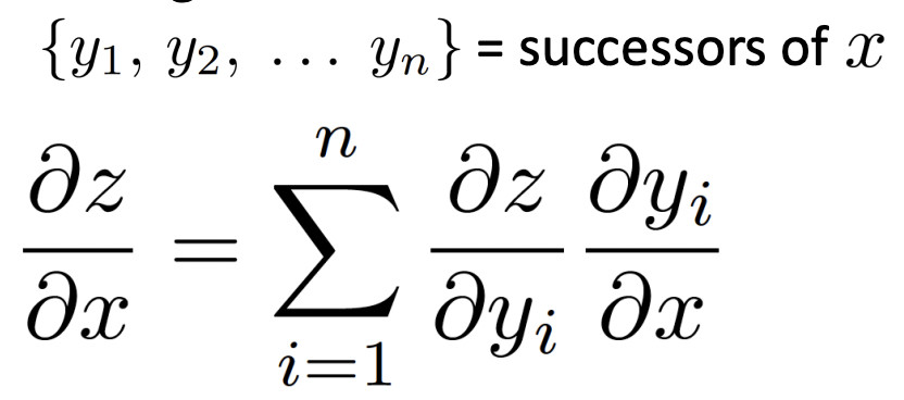
generalized form of the chain rule where we have multiple outputs
- forward propagation과 backpropagation의 big O complexity는 동일한다.
- 일반적으로 neural networks는 regular layer-structure를 가지고 있어 matrices와 Jacobians를 사용할 수 있고 parallel하게 훨씬 더 효율적으로 할 수 있다.
✔️ Automatic Differentiation
- 위 과정을 하는 것을 automatic differentiation이라고 한다.
Reference
- CS224n: Natural Language Processing with Deep Learning Lecture at Stanford University