0. Intro

Vectors

Definition

(1) 서로 더하거나 (2) scalar를 곱하여 같은 종류의 다른 객체를 생성할 수 있는 특수한 객체

Examples of vector objects

1. Geometric vectors (기하학적 벡터)
2. Polynomials (다항식)
3. Audio signals (음성 신호)
4. Elements of $\mathbb{R}^{n}$ (n개 실수의 tuple)

Linear Algebra는 이러한 벡터 개념 간의 유사성(similarities)에 집중

Closure

작은 벡터 집합에서 이들을 서로 더하거나 스케일링하여 얻을 수 있는 벡터 집합은 무엇인가?

Vector Space

Closure 연산을 통해서 vector space(벡터 공간)가 생성됨

1. Systems of Linear Equations

많은 문제들은 연립선형방정식(systems of linear equations)으로 공식화될 수 있고, 선형대수학은 이 문제들을 풀 수 있는 방법을 제공함

General form of a system of linear equations 👉 Example 2.1

• unknowns of this system : 구하고자 하는 변수
• solutions of this system : 해

일반적으로 실수 값에 대한 연립선형방정식에서 우리는 하나도 없거나, 오직 하나이거나, 무한히 많은 해를 얻음 👉 Example 2.2

• no solution
• unique solution
• infinitely many solutions(redundancy 발생)

Geometric Interpretation of Systems of Linear Equations

• two variables
  • 각 선형방정식은 line을 정의
  • solution set은 line, point, empty 중 하나
• three variables
  • 각 선형방정식은 plane을 정의
  • solution set은 plane, line, point, empty 중 하나

연립 선형 방정식을 풀기 위해 useful compact notation 도입 ➡️ matrices

2. Matrices

2.1 Matrix Addition and Multiplication

Matrix Operations

• element-wise sum
• A⋅B = multiplication = dot product
  • 교환법칙 성립 안됨 (not commutative) 👉 Example 2.3
• hadamard product = element-wise multiplication

Identity Matrix

Matrix Properties

• Associativity
  결합법칙 성립
• Distributivity
  분배법칙 성립
• Multiplication with the identity matrix
  identity matrix와 multiplication하면 자기자신

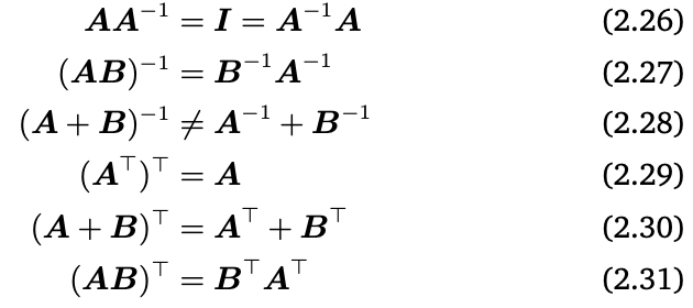
2.2 Inverse and Transpose

Inverse

모든 square matrix가 inverse를 가지고 있지 않음

Inverse 존재 의미

Square matrix에 대하여

• inverse가 존재
  • regular/invertible/nonsingular
  • unique하다고 말함
• inverse가 존재하지 않음
  • singular/noninvertible

역행렬(Inverse Matrix) 👉 Examples 2.4 (Inverse Matrix)

Transpose

열을 행으로 바꾼 것, 또는 그 반대
전치행렬(Transpose Matrix)

Important properties of inverses and transposes

Symmetric Matrix

• 자기 자신과 전치행렬이 같음
• square matrix만이 symmetric matrix가 될 수 있음
• A가 invertible하면 $A^{T}$도 invertible하고, $($$A^{-1}$$)^{T}$ = $($$A^{T}$$)^{-1}$ =: $A^{-T}$

Sum and Product of Symmetric Matrices

• 두 symmetric matrix의 sum은 항상 symmetric
• 두 symmetric matrix의 product는 일반적으로 not symmetric

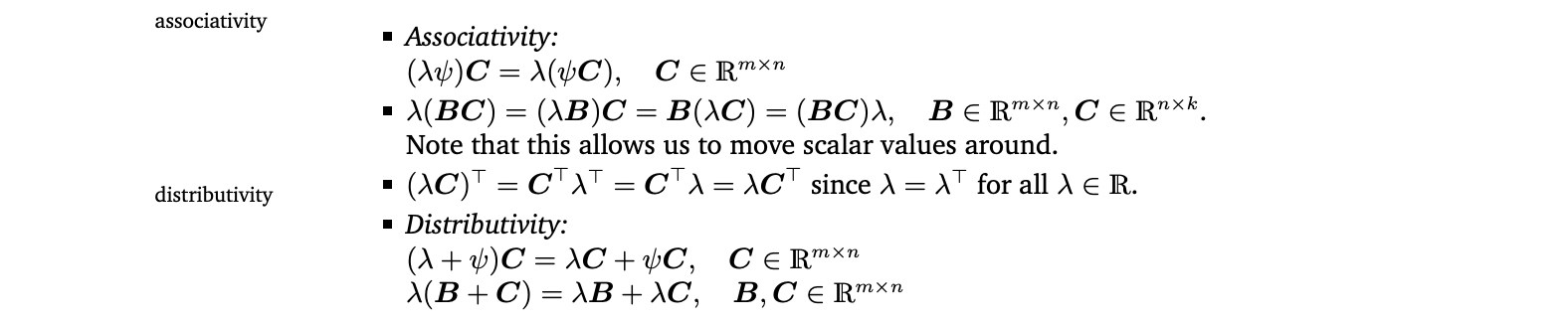
2.3 Multiplication by a Scalar

• Associativity
• Distributivity 👉 Example 2.5 (Distributivity)

2.4 Compact Representations of Systems of Linear Equations

다음과 같은 연립선형방정식이 있을 때,

Matrix multiplication을 사용하면 연립선형방정식을 다음과 같이 간략한 형태로 작성할 수 있음

• x1은 첫 번째 column을, x2는 두 번째 column을, x3는 세 번째 column을 scale함
• Ax = b
• Ax : linear combination of the columns of A

3. Solving Systems of Linear Equations

3.1 Particular and General Solution

• particular solution or special solution을 구하고 general solution을 구하는 일반적인 세 단계가 있음
  

• Gaussian elimination : 연립선형방정식을 simple form으로 바꾸는 constructive algorithmic 방법

  • gaussian elimination의 key는 연립선형방정식의 elementary transformations임

Gaussian elimination 방법을 사용해서 연립방정식을 simple form으로 바꾸고 그 다음, 세 단계를 적용

3.2 Elementary Transformations

elementary transformations

solution set은 같게 두면서, 연립방정식을 더 간단한 form으로 변환하는 것으로, 연립선형방정식을 풀 때 사용한다.

• 두 방정식을 바꿈
• constant를 방정식에 곱함
• 두 방정식을 더함

Elementary transformations를 사용해서 연립선형방정식 풀기 👉 Example 2.6

• compact matrix notion Ax = b
• augmented matrix [A|b]
• row-echelon form (REF)

Pivots

Leading coefficient of a row (왼쪽에서부터 0이 아닌 첫 번째 숫자)이며, 각 행의 pivot은 위에 있는 행의 pivot의 오른쪽에 위치한다.

Row-Echelon Form

• 0으로만 구성된 행이 행렬의 가장 아랫쪽에 위치 (0이 아닌 요소를 하나 이상 가지고 있는 행은 0으로만 구성된 행 위에 존재)
• 0이 아닌 행만 봤을 때, 왼쪽에서부터 처음으로 0이 아닌 숫자(pivot or leading coefficient)가 항상 그 행의 윗 행의 피벗의 오른쪽에 위치

Basic variables

Row-echelon form에서 pivot에 해당하는 variables

Free variables

그 외의 variables

Row-echelon form을 이용해서 particular solution 구하기

pivot columns를 사용하여 연립방정식의 오른쪽 부분을 표현. 가장 오른쪽에 있는 pivot column의 coefficient부터 시작하여 왼쪽으로 가면 쉽게 구할 수 있다. 이때 non-pivot columns의 coefficient는 0으로 둔 것임.

Reduced Row-Echelon form

• row-echelon form임
• pivot이 모두 1임
• 그 pivot의 column에서 해당 pivot을 제외한 나머지 entry는 0

Reduced row-echelon form으로 연립선형방정식의 general solution을 쉽게 구할 수 있음 👉 Example 2.7 (Reduced Row Echelon Form)

Gaussian elimination

연립선형방정식을 reduced row-echelon form으로 변환하기 위해 elementary transformations를 수행하는 알고리즘

3.3 The Minus-1 Trick

Reduced row echelon form에서 general solution을 쉽게 구하게 해주는 trick
👉 Example 2.8 (Minus-1 Trick)

kenel or null space

solution space of homogeneous equation system Ax = 0

Calculating the Inverse

👉 Example 2.9 (Calculating an Inverse Matrix by Gaussian Elimination)
Augmented equation system([A|I])을 reduced REF로 바꾸면 연립방정식의 오른쪽 부분이 inverse임

3.4 Algorithms for Solving a System of Linear Equations

• Matrix가 invertible하면 x = $A^{-1}b$ 가 solution
• 일반적인 경우 gaussian elimination 사용

4. Vector Spaces

4.1 Groups

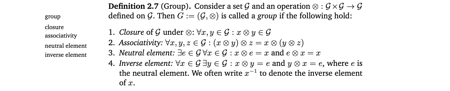
👉 Example 2.10 (Groups)

Abelian group

group인데 교환법칙도 성립하면 abelian group

General Linear Group

Regular(invertible) matrices 집합은 matrix multiplication 연산에 대해서 group GL(n,R)을 이룸.
(matrix multiplication이 교환법칙은 성립하지 않으므로 abelian group은 아님)

4.2 Vector Spaces

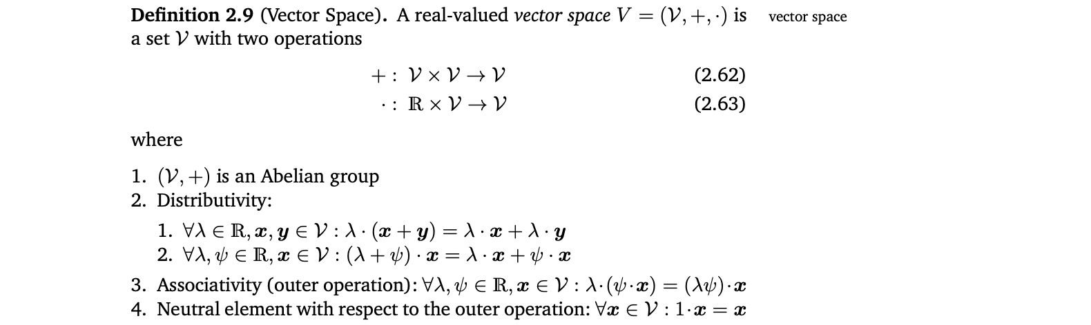
• Vector space V 의 element : vector
• Neutral element of (V,+) : zero vector
• inner operation of (V,+) : vector addition
• λ : scalars
• outer operation : multiplication by scalars

👉 Example 2.11 (Vector Spaces)

Notation

• V : +가 standard vector addition이고 ⋅가 scalar multiplication일 때의 vector space (V,+,⋅)
• x : column vector (element in the vector space $R^{n}$)

• $x^{T}$ : row vector (the transpose of x, element in the vector space $R^{1×n}$)

4.3 Vector Subspaces

Vector subspace는 다음 조건을 만족해야한다.

• 모든 subspace U⊆($R^{n}$,+,⋅) 은 homogeneous system of linear equations Ax=0 (x∈$R^{n}$) 의 solution space이다.

👉 Example 2.12 (Vector Subspaces)

5. Linear Independence

Linear Combination

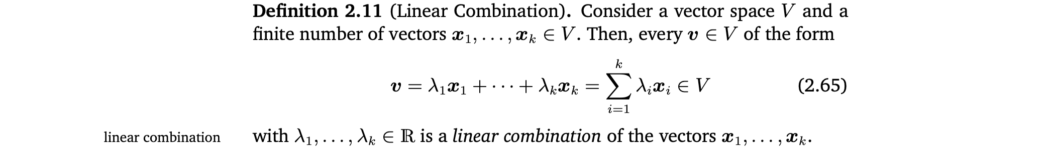
0-vector는 항상 k개의 vector의 linear combination으로 나타낼 수 있음. 0을 표현할 수 있는, vector집합의 non-trivial combinations에 관심있음.(즉, (2.65)에서 모든 coefficients가 0이 아님)

Linear (In)dependence

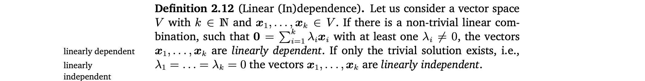
• 이러한 non-trivial linear combination이 있으면 그 vector들은 linearly dependent하다고 함.
• 만약 오직 Trivial solution만 존재하면 그 vector들은 linearly independent하다고 함.

Linear independence는 선형대수학에서 가장 중요한 개념 중 하나이다. linearly independent한 vector의 집합에서 vector를 하나라도 빼면 정보를 잃는 것

👉 Example 2.13 (Linearly Dependent Vectors)

• Linearly independent를 체크하는 법 👉 Example 2.14

  • k vectors는 linearly dependent하거나 linearly independent함. 둘 중 하나임.
  • 하나라도 0-vector이거나, 두 vector가 같으면 linearly dependent함.
  • 한 vector가 다른 vector의 배수이면 그 집합은 linearly dependent함.
  • vector들을 column으로 하여 matrix A를 만들고 matrix가 row echelon form이 될 때까지 Gaussian elimination 수행. 만약 모든 column이 pivot column이면 모든 column vector들은 linearly independent하며, 하나라도 non-pivot column이 있으면 그 column vector들(corresponding vectors)은 linearly dependent함.

• k개의 linearly independent vectors가 있고 m개의 linear combinations가 있을 때 x 집합이 linearly independent한지 아는 방법 👉 Example 2.15

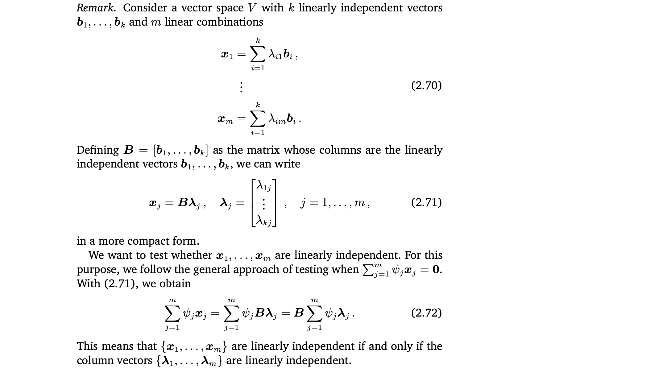
• column vectors가 linearly independent해야한다.
• m>k이면 x 집합은 linearly dependent

6. Basis and Rank

6.1 Generating Set and Basis

Generating set
Span

Minimal
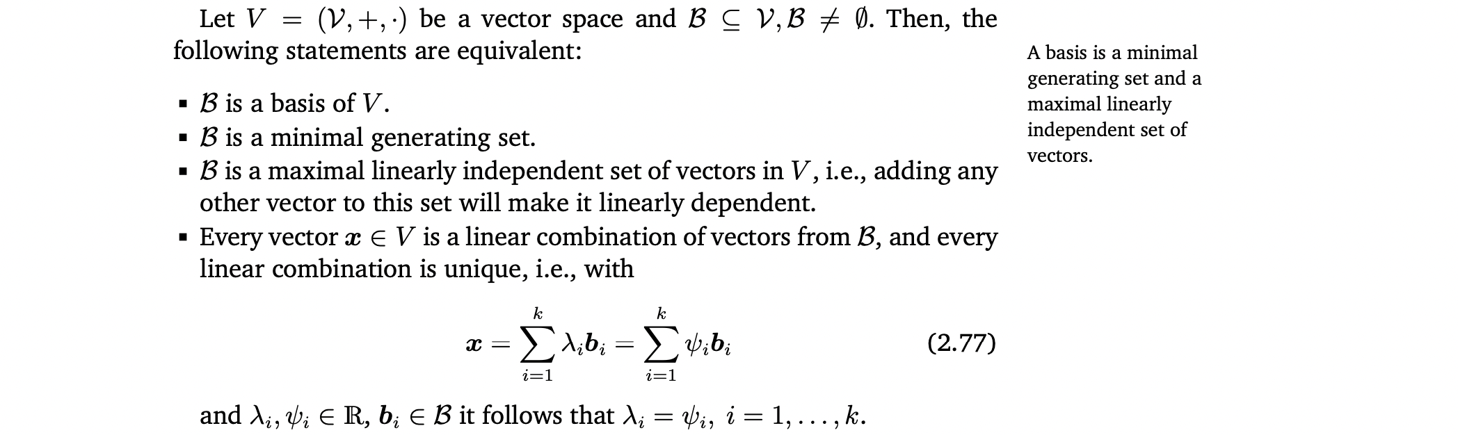
Basis : minimal generating set이자 maximal linearly independent set of vectors임 👉 Example 2.16

👉 Example 2.16

• 모든 vector space는 basis를 가지고 있음
• Vector space는 여러개의 basis를 가질 수 있음
• 하지만 그 basis를 이루는 vector의 수는 항상 같음
• dimension of V = the number of basis vectors of V = dim(V)
• 만약 U⊆V가 V의 subspace이면, dim(U)≤dim(V)이다. 그리고 U=V일때만 dim(U)=dim(V)이다.
• 직관적으로 vector space의 dimension은 vector space에서 independent directions의 개수로 생각할 수 있음
• vector space의 dimension이 vector 안의 element 수와 같을 필요는 없다.
• Basis 찾는 법 👉 Example 2.17 (Determining a Basis)
  

6.2 Rank

Matrix A ∈ $R^{m×n}$ 에 대하여
linearly independent columns의 개수 = linearly independent rows의 개수 = rank of A = rk(A)이다.

image or range
kernel or null space
full rank ↔️ rank deficient

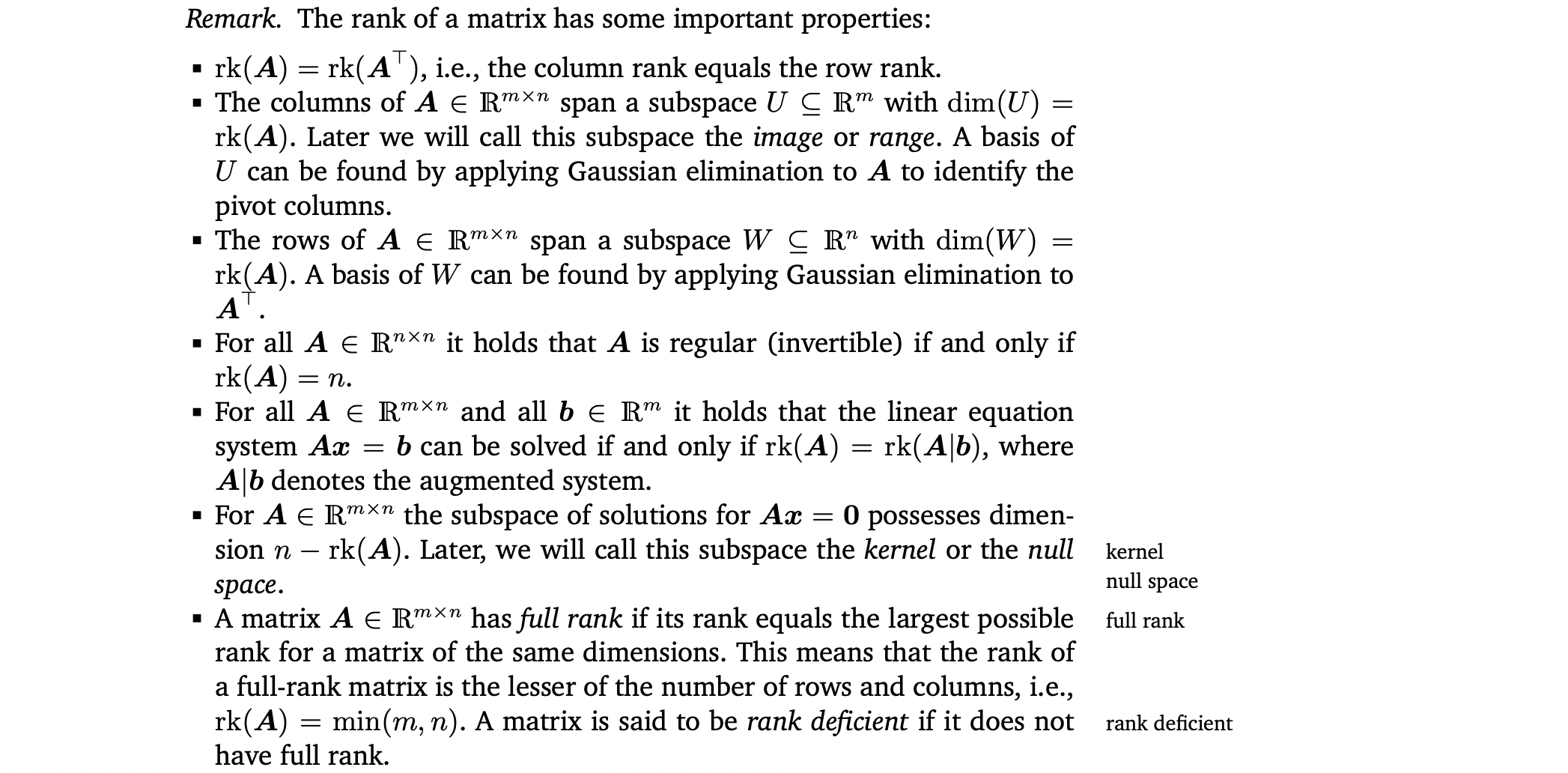
• Matrix A의 rank 구하기 👉 Example 2.18 (Rank)

7. Linear Mappings

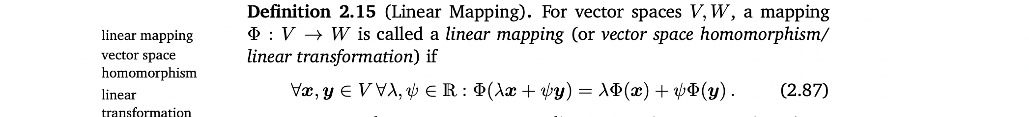
Mapping을 한 후에도 vector space의 structure(더하거나 Scalar를 곱해도 여전히 vector)를 보존해야함
linear mapping = vector space homomorphism = linear transformation 👉 Example 2.19 (Homomorphism)

• linear mapping을 matrices로 표현할 수 있음
• Matrix가 linear mapping을 표현하는지, collection of vectors를 표현하는지 알고 있어야함.

Special mappings(Injective, Surjective, Bijective)

• mapping이 surjective하면, W 안의 모든 element는 mapping을 사용하여 V로부터 "reached"할 수 있음(즉, 공역=치역).
• mapping이 bijective하면 "undone"할 수 있음. 즉, inverse mapping이 존재

Special cases of linear mappings

Isomorphism
Endomorphism
Automorphism
Identity mapping or identity automorphism

Isomorphic

• Theorem 2.17은 같은 차원의 두 vector spaces간에는 linear, bijective mappping이 존재한다는 것을 말함. 즉, 손실없이 서로 변환될 수 있기 때문에 같은 차원의 vector spaces들은 서로 같은 종류의 것이라는 것을 의미함.

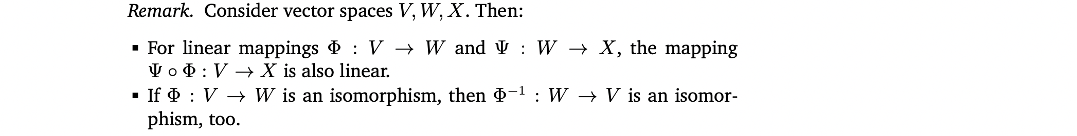
Linear mapping 성질

7.1 Matrix Representation of Linear Mappings

Ordered basis

n차원 벡터는 $R^{n}$에 isomorphic함.
n차원 vector space V의 basis {$b_{1}$...$b_{n}$}가 있을 때, basis의 순서가 중요
B = ($b_{1}$...$b_{n}$) 라는 n tuple을 ordered basis of V라고 함.

Notation

• ordered basis B = ($b_{1}$...$b_{n}$)
• (unordered) basis B = {$b_{1}$...$b_{n}$}
• $b_{1}$...$b_{n}$를 column으로 가지는 matrix B = [$b_{1}$...$b_{n}$]

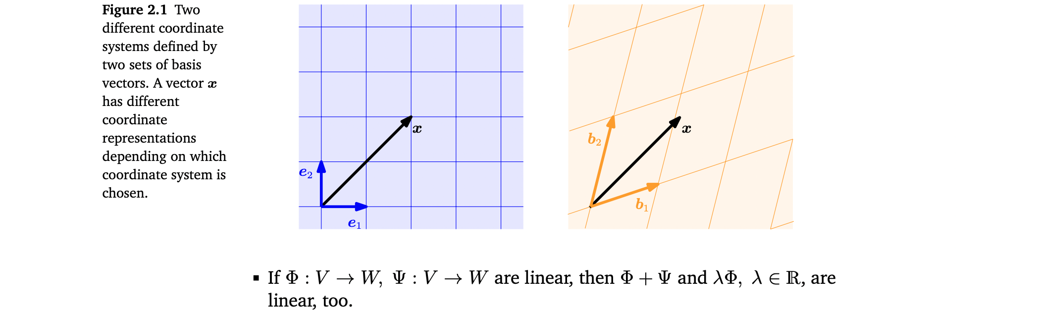
Coordinates

coordinates
coordinate vector/coordinate representation of x

• basis가 무엇인가에 따라 같은 vector x가 다른 coordinate representation을 가질 수 있음 👉 Example 2.20
• Cartesian coordinate system의 basis는 canonical basis vectors $e_{1}$, $e_{2}$

Transformation Matrix

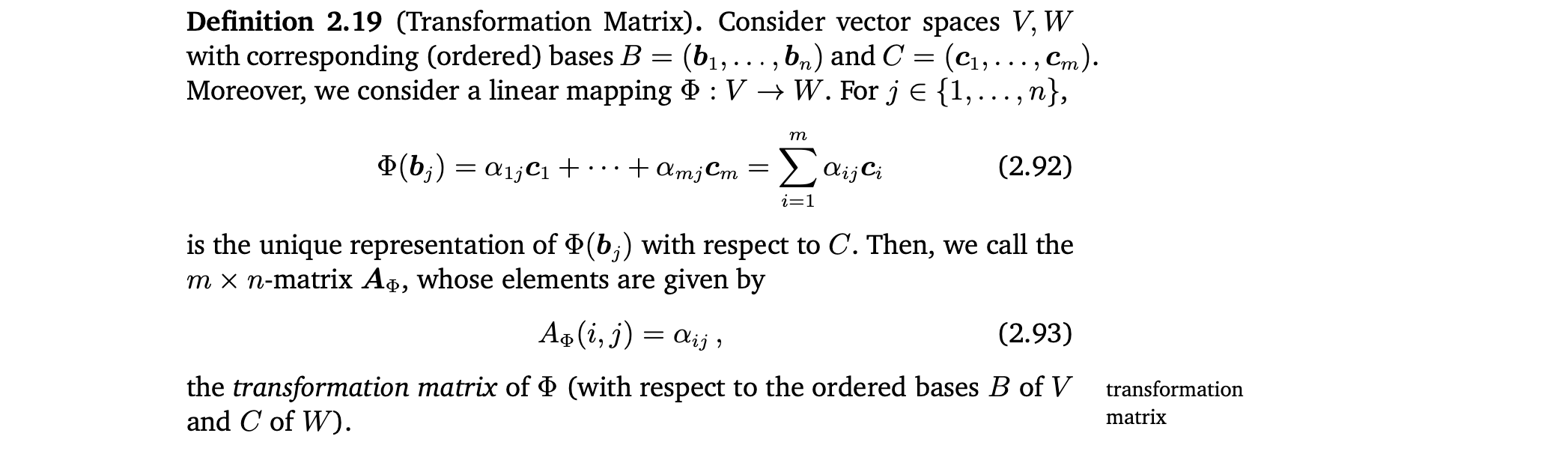
• W의 ordered basis C에 대한 Φ($b_{j}$)의 coordinates는 transformation matrix $A_{Φ}$의 j번째 column임.

Transformation matrix 구하기 👉 Example 2.21(Transformation Matrix)

• transformation matrix는 V의 ordered basis에 대한 coordinates를 W의 ordered basis에 대한 coordinates로 mapping하는 데 사용될 수 있음.

Linear Transformations of Vectors 👉 Example 2.22(Linear Transformations of Vectors)

7.2 Basis Change

만약 V와 W의 basis를 바꾸면 linear mapping Φ : V -> W 의 transformation matrix는 어떻게 바뀔까?

Example 2.23(Basis Change)

Basis Change

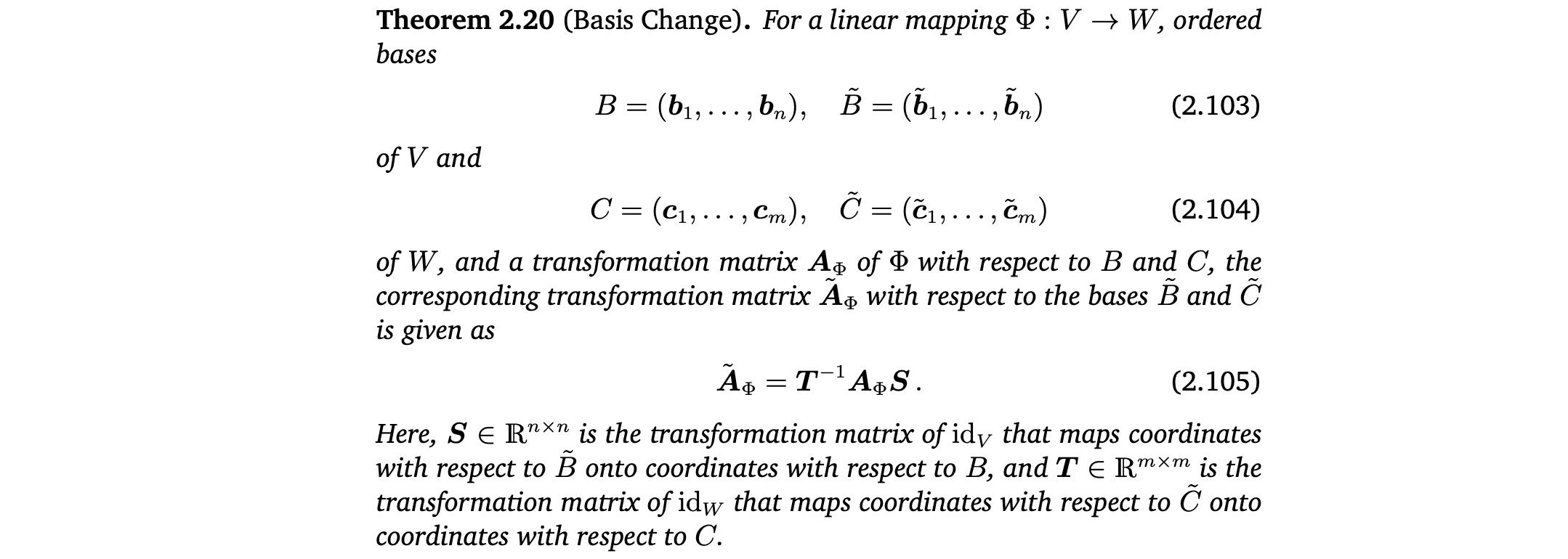
Ordered basis B, C에 대한 $Φ_{CB}$ mapping의 transformation matrix $A_{Φ}$를 안다고 가정. Basis B와 C를 변경했을 때 그것에 해당하는 transformation matrix를 구하는 방법 👉 Example 2.24 (Basis Change)

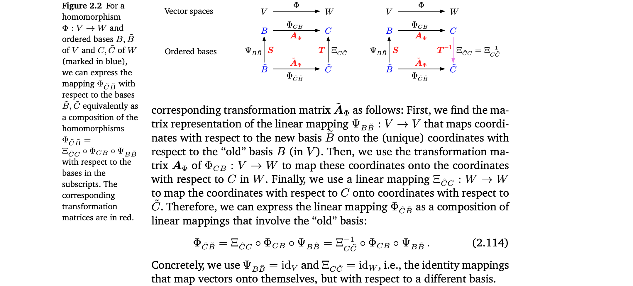
1. new basis B에 대한 coordinates를 old basis B에 대한 coordinates로 mapping하는 linear mapping의 matrix representation을 찾는다.
2. $Φ_{CB}$ 사용
3. old basis C에 대한 coordinates를 new basis C에 대한 coordinates로 mapping하는 linear mapping을 구한다.

Equivalence

Similarity

Similar matrices는 항상 equivalent함. 하지만 반대는 항상 성립하지 않음

(2.116)에서 계산은 오른쪽에서 왼쪽으로 해야함. 왜냐하면 vector가 오른쪽에서 곱해지기 때문이다.

7.3 Image and Kernel

Image and Kernel

Linear mapping의 image와 kernel은 중요한 특정 성질을 가진 vector subspaces이다.

kernel/null space
image/range
domain
codomain

• kernel : Φ가 neutral element $0_{W}$ ∈ W 에 mapping하는 vectors v ∈ V 의 집합
• image : V에 있는 vector로부터 Φ에 의해 "reached"할 수 있는 vectors w ∈ W 의 집합

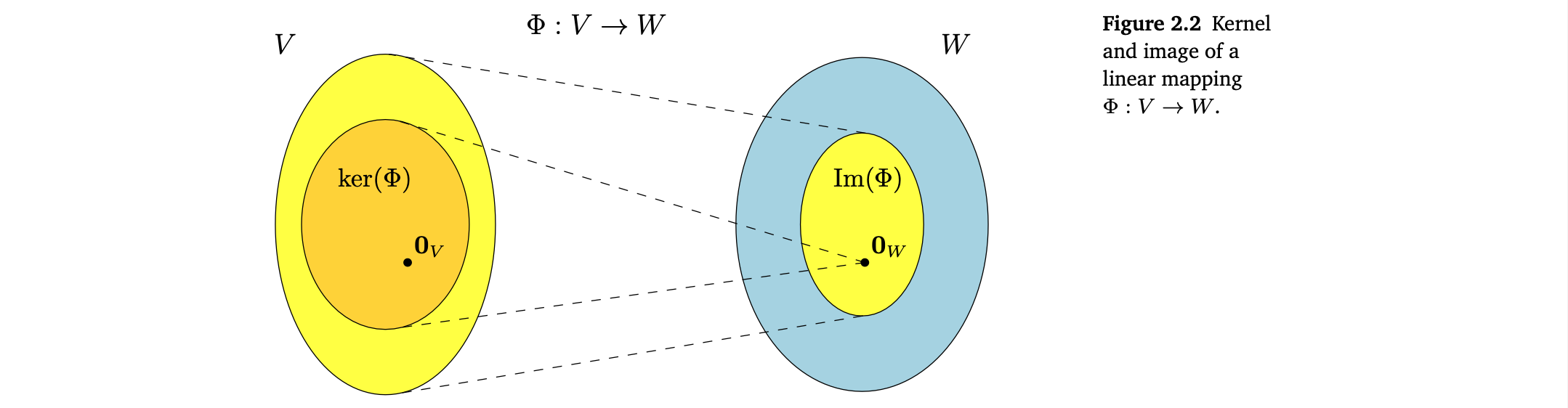
• $Φ(0_{V}) = 0_{W}$, 그러므로 0_{V} ∈ ker($Φ$). 특히, null space는 절대 empty가 아님.
• Im($Φ$) ⊆ W 는 W의 subspace, ker($Φ$) ⊆ V 는 V의 subspace
• 'ker($Φ$) = {0}'은 '$Φ$는 injective (one-to-one mapping)'의 필요충분조건이다.

Null Space and Column Space

• column space = image Im($Φ$) = span of the columns of A
  • column space(image)는 $R^{m}$의 subspace
• rk(A) = dim(Im($Φ$))
• kernel/null space ker($Φ$) = homogeneous system of linear equations Ax=0의 general solution
  • 0∈$R^{m}$을 만들어내는 $R^{n}$의 모든 요소들의 linear combinations를 포착함.
  • kernel은 $R^{n}$의 subspace
• kernel은 column들간의 관계에 중점을 두고 있으며, 이를 활용하여 한 column을 다른 column들의 linear combination으로 표현할 수 있는지, 어떻게 표현하는지 확인할 수 있음.

👉 Example 2.25(Image and Kernel of a Linear Mapping)

Rank-Nullity Theorem

fundamental theorem of linear mappings라고 부르기도 함.

위 theorem에 의해 다음과 같은 성질을 가지고 있음 ????

8. Affine Spaces ??

원점에서 offset이 되는 공간. 더이상 vector의 subspace가 아님.

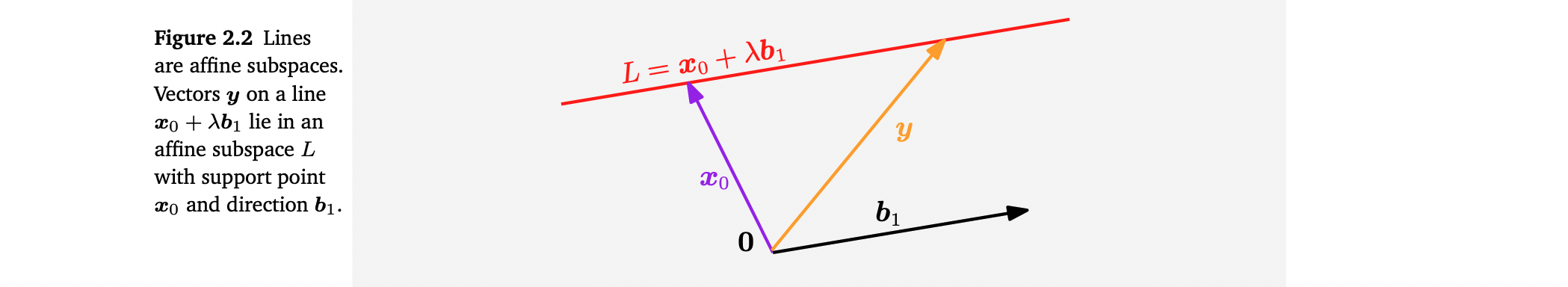
Affine Subspace

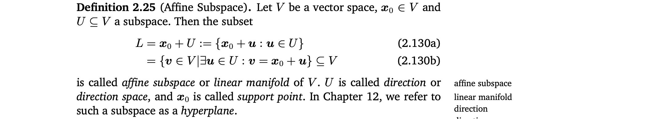
• L : affine subspace or linear manifold of V
• U : direction or direction space
• $x_{0}$ : support point

Chapter 12에서는 이 subspace를 hyperplane이라고 말함.

Affine subspace는 $x_{0}$ ∉ U 이면 0을 제외하게 됨. 그래서 affine subspace는 V의 (linear) subspace (vector subspace)가 아님.

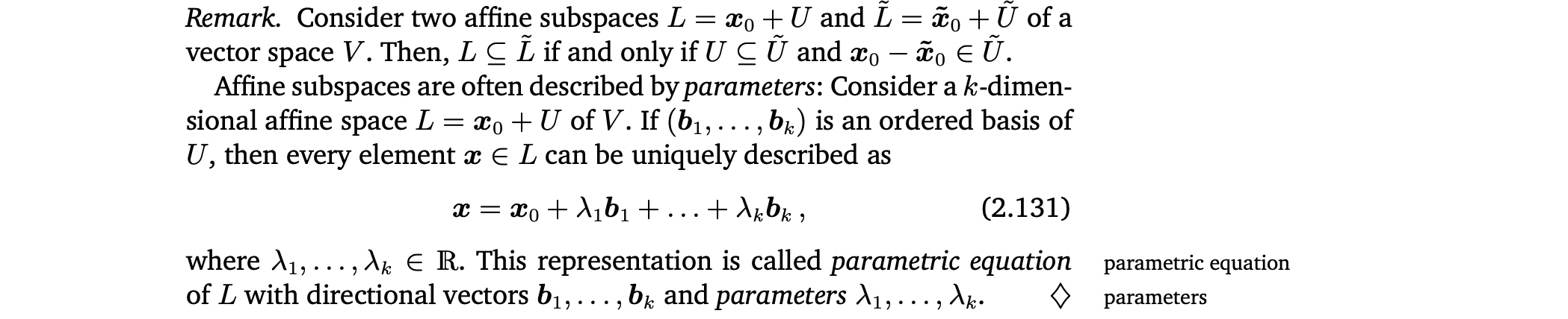
Parametric equation of affine subspace

parameteric equation
parameters

Inhomogeneous systems of linear equations and affine subspaces

• A ∈ $R^{m×n}$, x ∈ $R^{m}$에 대하여 연립선형방정식 Aλ=x의 해는 empty set 또는 dimension이 n-rk(A)인 $R^{n}$의 affine subspace임. 특히 ($λ_{1}$ , ... , $λ_{1}$) ≠ (0, ..., 0) 인 해는 $R^{n}$에서 hyperplane임.
• $R^{n}$에서 모든 k-dimensional affine subspace는 inhomogeneous system of linear equations Ax=b의 solution이고, A ∈ $R^{m×n}$, b ∈ $R^{m}$, rk(A)=n-k임.
• homogeneous equation systems Ax=0의 solution은 vector subspace인데, support point $x_{0}=0$인 special affine space로 생각할 수 있음.

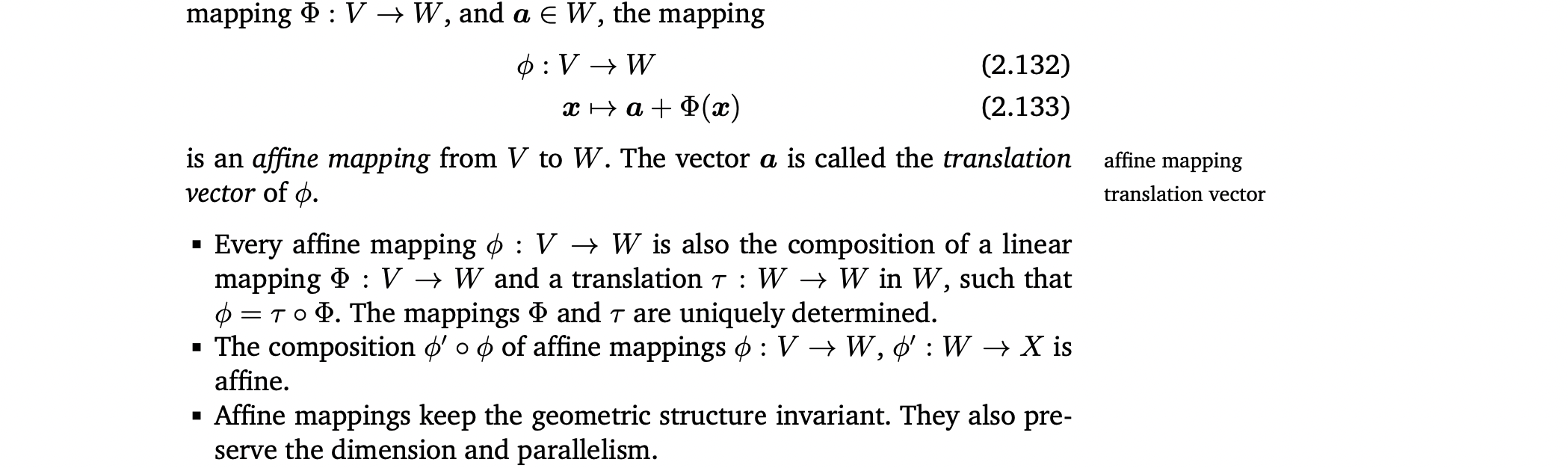
8.2 Affine Mappings

translation vector