---

[이미지 처리 바이블] 교재 4장을 기반으로 작성되었습니다.

---

4.3 비전 트랜스포머

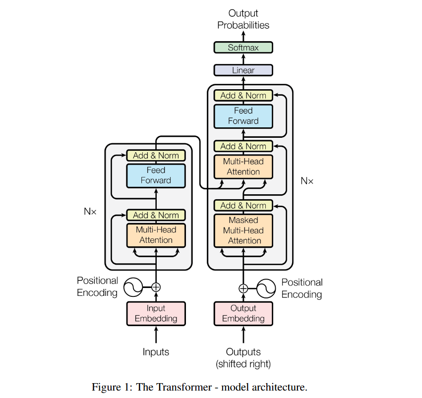
4.3.1 트랜스포머

Transformer란 딥러닝 모델 중 하나로, 자연어 처리에서 좋은 성능을 내고 있는 모델 구조임
이 모델을 이미지 처리에 적용하기 위해 만들어진 모델이 Vision Transformer

Google Brain 팀이 2017년에 발표한 트랜스포머 논문에 대한 설명은 아래 링크 참조
[논문리뷰] Attention is All you Need

---

어텐션

Attnetion 매커니즘은 트랜스포머에서 가장 중요한 개념 중 하나
> 모델이 입력 데이터의 중요한 부분에 집중하도록 함 (어떻게?)

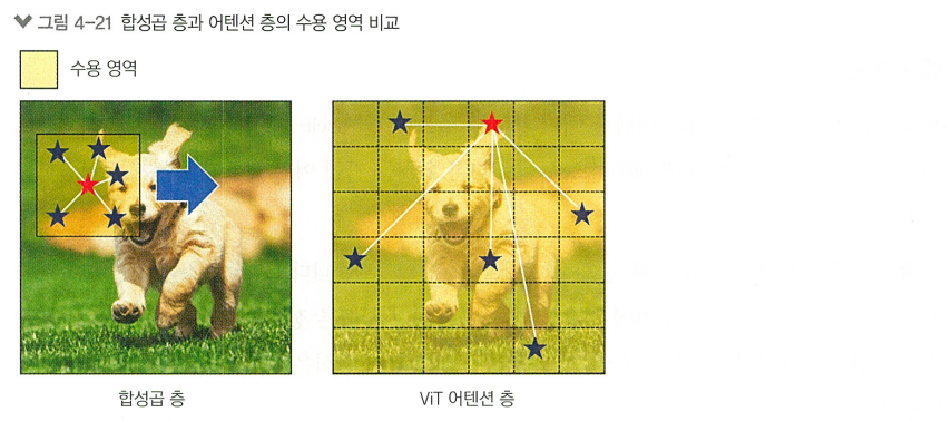
CNN은 하나의 작은 윈도우를 전체 이미지에서 옮겨가며 데이터를 읽기 때문에, 공간적 근접성의 귀납적 편향을 가지고 있음
> CNN은 지역적 패턴과 텍스처를 효율적으로 인식하도록 설계됨

ViT는 이미지를 여러 작은 조각(패치)로 분할하고, 이 패치들 간의 관계를 직접 모델링함.
> 이미지 전체의 전역적 컨텍스트 이해에 유리

>> 둘은 서로 다른 유형의 문제에 더 적할 수 있음

---

셀프 어텐션

셀프 어텐션은 주어진 입력에 대해 내부적으로 서로 다른 위치들 간에 어떤 관계가 있는지를 학습
기존의 seq2seq 모델은 입력 데이터의 순서, 위치에 의존하기 때문에, 문장이 길어질 수록 초반 입력 정보가 사라지는 문제(vanishing gradient problem)이 있었음

셀프 어텐션은 '어텐션' 방식을 사용해 위 문제를 해결함.
이는 seq2seq처럼 순차적으로 처리할 필요없이, 입력 데이터를 병렬 구조로 처리해 문장이 길어져 정보들이 멀어져도 연관성을 이끌어낼 수 있음

$Q, K, V$ 는 어디서 오는가?

$Q=XW_Q,\quad K=XW_K,\quad V=XW_V$

입력인 단어(토큰) 시퀀스는 임베딩 레이어를 거치면 임베딩 벡터로 변환되고,
Positional Encoding이 더해지면 입력 벡터 $X$로 전환됨.

이 입력 벡터에 각각의 가중치 행렬 $W_Q, W_K, W_V$ 를 곱하면 그제서야 $Q, K, V$ 가 됨!
(이 작업은 Multi-Head Attention 하단의 Linear 블록에서 이루어짐)

$W_Q, W_K, W_V$는 Transformer 모델이 처음 시작될 때 무작위로 초기화 되고, 훈련 과정을 거치면서 자동으로 업데이트 됨

$Q, K, V$ 각각의 역할

• $Q$ = Query: 현재 단어가 "어떤 단어를 참고해야 하는지" 결정하는 역할
• $K$ = Key: 각 단어가 자기 자신을 설명하는 정보
• $V$ = Value: 최종적으로 참고할 정보

즉, Query와 Key를 비교해서 "어떤 단어를 참고해야 하는지"를 결정하고
실제 정보는 Value에서 가져오는 것!

---

트랜스포머 모델 구조

---

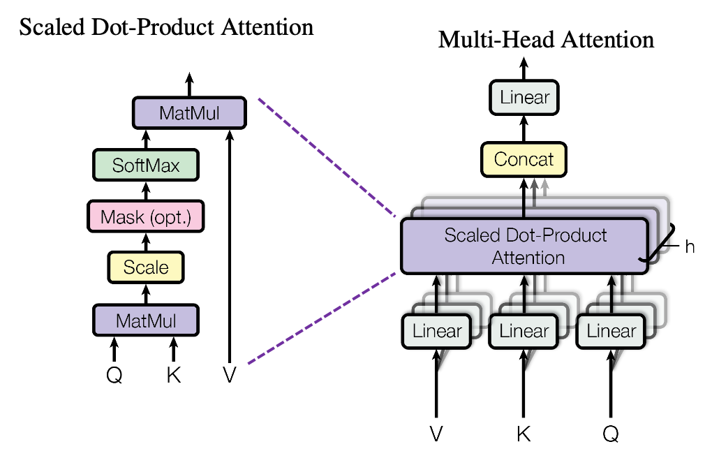
다중 헤드 어텐션

Attention을 여러 번 병렬로 수행하는 것을 의미함
> 입력 데이터의 서로 다른 특성을 동시에 모델링할 수 있게함

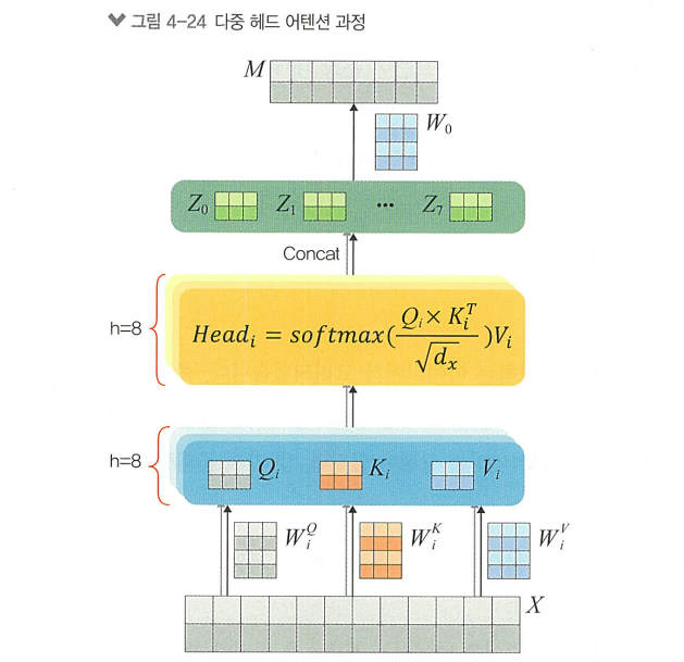
1. 선형 변환: 입력 $Q, K, V$는 각각의 가중치 행렬 $W_Q, W_K, W_V$ 사용해 h번 변환됨
2. 병렬 어텐션 계산: 변환된 $Q, K, V$에 대해 독립적인 어텐션을 수행함
3. 결합 및 최종 선형 변환: 각각의 어텐션의 출력 결합, 추가적인 가중치 행렬 $W_o$를 사용해 최종 결과 생성

> 여러개의 헤드(h)를 통해 입력 시퀀스의 다양한 부분에서 더 풍부한 정보를 추출하고 모델의 표현력을 향상시킴
> 서로 다른 위치의 정보를 동시에 고려해 문맥에 대한 이해를 향상시킴

---

포지셔널 인코딩

Positional Encoding은 입력의 토큰이 문장에서 갖는 위치 정보를 모델이 이해하기 위해 중요한 기법

1. 선형 포지셔널 인코딩
2. 정규화된 선형 포지셔널 인코딩
3. sin, cos 함수의 도입
   - 주기성: 주기적인 패턴을 가지고 있어, 어느 시퀀스를 처리하던 일관된 방식으로 인코딩 가능
   - 상대적 위치 정보: 각 위치 간의 상대적 차이를 유지할 수 있음
   - 차원 독립성: 다양한 주파수의 함수를 사용함으로써 모델이 다른 차원에서 위치 정보를 독립적으로 인코딩 가능
   
   

포지셔널 인코딩의 원리

• $pos$: 단어의 위치
• $i$: 차원의 인덱스
• $d_model$: 모델의 임베딩 차원
  
  

포지셔널 인코딩의 특징

• 순서 정보의 제공: 문장 내에서 단어의 위치 정보를 고려할 수 있게 함
• 학습이 필요 없는 고정된 인코딩: 학습 파라미터가 아닌, 미리 정의된 함수에 의해 생성되므로 모델에 부담이 덜함
• 길이 제한: 미리 정의된 최대 시퀀시 길이에 제한됨. 이를 위한 연구는 진행중

---

4.3.2 비전 트랜스포머

ViT

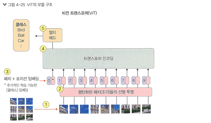
1. 자연어의 문장이 아닌 이미지를 처리하기 위해, 입력 이미지를 NxN의 작은 정사각형 조각(patch)으로 쪼갬
2. 각 NxN의 patch를 flatten하여 1차원 벡터로 변환
3. 이미지의 위치 정보를 모델에게 제공하기 위해 Position Embedding하고, 분류 작업을 위해 입력 스퀀스의 맨 앞에 특별한 [CLS] 토큰을 추가함. 이 토큰은 모델을 통과하며 전체 이미지에 대한 정보를 집약함
4. 임베딩 된 patch는 ViT의 트랜스포머 인코더 블록의 입력으로 들어가 Multi-Head Attention을 통해 서로 다른 이미지 patch에서의 관련성을 학습함 (기존 Transformer와 정규화 위치 빼곤 차이 X)
5. 인코더를 통과한 [CLS] 토큰의 출력은 이미지 전체를 대표하는 고차원 특징 벡터가 됨. 이 벡터가 MLP Head의 입력으로 들어가 모델의 최종 출력을 생성함

---

ViT 모델 구현 실습

import numpy as np
import tensorflow as tf
import matplotlib.pyplot as plt
from tensorflow.keras import layers

""" 📌 cifar100 데이터셋 로드 """
(train_x, train_y), (test_x, test_y) = tf.keras.datasets.cifar100.load_data()
num_classes = 100

plt.figure(figsize=(10, 2))
for i in range(5):
    plt.subplot(1, 5, i + 1)
    plt.imshow(train_x[i])
    plt.title(f"Label: {train_y[i][0]}")
    plt.axis('off')
plt.show()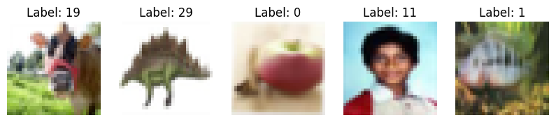

""" 📌 정규화 """
print(f"스케일링 전 픽셀의 최대 값과 최소 값:{train_x.min()} ~ {train_x.max()}")
train_x = train_x/255.
test_x = test_x/255.
print(f"스케일링 후 픽셀의 최대 값과 최소 값:{train_x.min()} ~ {train_x.max()}")

>>> 스케일링 전 픽셀의 최대 값과 최소 값:0 ~ 255
	스케일링 후 픽셀의 최대 값과 최소 값:0.0 ~ 1.0

""" 📌 모델 파라미터 정의 """
input_shape = (32, 32, 3)
batch_size = 64   		# 트랜스포머는 대규모 병렬 처리가 용이하므로 배치 사이즈를 더 키워보는 것이 좋음

image_size = 72   		# 패치 분할을 위해 입력 이미지를 재조정할 사이즈
patch_size = 6
num_patches = (image_size // patch_size) ** 2   # 이미지에서 분할되는 patch의 총 개수

learning_rate = 1e-3
weight_decay = 1e-4   	# 가중치 감소 규제 기법의 파라미터
epochs = 30

transformer_layers = 4  # 트랜스포머 내부의 인코더 레이어 수
projection_dim = 64   	# 패치를 투영할 때의 차원 수
num_heads = 4			# Multi-Head Attention에서의 헤드 수 (h)
transformer_units = [projection_dim * 2, projection_dim]   # 트랜스포머의 FFN에서 사용되는 유닛의 수
mlp_head_units = [2048, 1024]   # 최종 부분의 MLP의 유닛 수

""" 📌 이미지 patch를 만들어주는 클래스 정의 """
class PatchTokenization(layers.Layer):
    def __init__(self, image_size=image_size, patch_size=patch_size, num_patches=num_patches, projection_dim=projection_dim, **kwargs):
        super().__init__(**kwargs)
        self.image_size = image_size
        self.patch_size = patch_size
        self.half_patch = patch_size // 2
        self.flatten_patches = layers.Reshape((num_patches, -1))   # patch 평탄화
        self.projection = layers.Dense(units=projection_dim)       # patch 투영 (고정된 사이즈의 벡터로 매핑)
        self.layer_norm = layers.LayerNormalization(epsilon=1e-6)  # 레이어 정규화

    def call(self, images):
        patches = tf.image.extract_patches(
            images=images,
            sizes=[1, self.patch_size, self.patch_size, 1],
            strides=[1, self.patch_size, self.patch_size, 1],
            rates=[1, 1, 1, 1],
            padding="VALID",
        )
        flat_patches = self.flatten_patches(patches)
        tokens = self.projection(flat_patches)
        return (tokens, patches)

""" 📌 이미지 patch 시각화 """
image = train_x[np.random.choice(range(train_x.shape[0]))]
resized_image = tf.image.resize(tf.convert_to_tensor([image]), size=(image_size, image_size))

(token, patch) = PatchTokenization()(resized_image)
(token, patch) = (token[0], patch[0])
n = patch.shape[0]
count = 1
plt.figure(figsize=(4, 4))
for row in range(n):
    for col in range(n):
        plt.subplot(n, n, count)
        count = count + 1
        image = tf.reshape(patch[row][col], (patch_size, patch_size, 3))
        plt.imshow(image)
        plt.axis("off")
plt.show()

""" 📌 patch 인코더 클래스 정의 """
class PatchEncoder(layers.Layer):
    def __init__(self, num_patches=num_patches, projection_dim=projection_dim, **kwargs):
        super().__init__(**kwargs)
        self.num_patches = num_patches
        self.position_embedding = layers.Embedding(input_dim=num_patches, output_dim=projection_dim)  
        self.positions = tf.range(start=0, limit=self.num_patches, delta=1)

    def call(self, encoded_patches):
        encoded_positions = self.position_embedding(self.positions)
        encoded_patches = encoded_patches + encoded_positions
        return encoded_patches

""" 📌 MLP 클래스 정의 """
def mlp(x, hidden_units, dropout_rate):
    for units in hidden_units:
        x = layers.Dense(units, activation=tf.nn.gelu)(x)
        x = layers.Dropout(dropout_rate)(x)
    return x

""" 📌 ViT 이미지 분류기 생성 함수 정의 """
def create_vit_classifier():
    inputs = layers.Input(shape=input_shape)
    x = layers.Normalization()(inputs)
    x = layers.Resizing(image_size, image_size)(x)
    (tokens, _) = PatchTokenization()(x)
    encoded_patches = PatchEncoder()(tokens)
    for _ in range(transformer_layers):
        x1 = layers.LayerNormalization(epsilon=1e-6)(encoded_patches)
        attention_output = layers.MultiHeadAttention(num_heads=num_heads, key_dim=projection_dim, dropout=0.1)(x1, x1)
        x2 = layers.Add()([attention_output, encoded_patches])
        x3 = layers.LayerNormalization(epsilon=1e-6)(x2)
        x3 = mlp(x3, hidden_units=transformer_units, dropout_rate=0.1)
        encoded_patches = layers.Add()([x3, x2])

    x = layers.LayerNormalization(epsilon=1e-6)(encoded_patches)
    x = layers.Flatten()(x)
    x = layers.Dropout(0.5)(x)
    x = mlp(x, hidden_units=mlp_head_units, dropout_rate=0.5)
    outputs = layers.Dense(num_classes)(x)
    model = tf.keras.Model(inputs=inputs, outputs=outputs)
    return model

""" 📌 CosineDecay 클래스 정의 """
# 학습률 조정 방법 중 하나
class CosineDecay(tf.keras.optimizers.schedules.LearningRateSchedule):
    def __init__(self, learning_rate_base, total_steps, warmup_learning_rate, warmup_steps):
        super().__init__()
        self.learning_rate_base = learning_rate_base
        self.total_steps = total_steps
        self.warmup_learning_rate = warmup_learning_rate
        self.warmup_steps = warmup_steps
        self.pi = tf.constant(np.pi)

    def __call__(self, step):
        if self.total_steps < self.warmup_steps:
            raise ValueError("total_steps 값이 warmup_steps보다 크거나 같아야합니다.")

        cos_annealed_lr = tf.cos(self.pi * (tf.cast(step, tf.float32) - self.warmup_steps) / float(self.total_steps - self.warmup_steps))
        learning_rate = 0.5 * self.learning_rate_base * (1 + cos_annealed_lr)

        if self.warmup_steps > 0:
            if self.learning_rate_base < self.warmup_learning_rate:
                raise ValueError(
                    "learning_rate_base 값이 warmup_learning_rate보다 크거나 같아야합니다.")
            slope = (self.learning_rate_base - self.warmup_learning_rate) / self.warmup_steps
            warmup_rate = slope * tf.cast(step, tf.float32) + self.warmup_learning_rate
            learning_rate = tf.where(step < self.warmup_steps, warmup_rate, learning_rate)
        return tf.where(step > self.total_steps, 0.0, learning_rate, name="learning_rate")

# CosineDecay 스케줄러 인스턴스 생성
total_steps = int((len(train_x) / batch_size) * epochs)
warmup_epoch_percentage = 0.10
warmup_steps = int(total_steps * warmup_epoch_percentage)
scheduled_lrs = CosineDecay(
    learning_rate_base=learning_rate,
    total_steps=total_steps,
    warmup_learning_rate=0.0,
    warmup_steps=warmup_steps,)

모델의 구성 단계

""" 📌 ViT 분류기 생성 & 모델 컴파일 """
vit = create_vit_classifier()

optimizer = tf.keras.optimizers.AdamW(
    learning_rate=scheduled_lrs,   # CosinDecay 학습률 스케줄러 사용
    weight_decay=weight_decay)

vit.compile(
    optimizer=optimizer,
    loss=tf.keras.losses.SparseCategoricalCrossentropy(from_logits=True),
    metrics=[tf.keras.metrics.SparseCategoricalAccuracy(name="accuracy"),
             tf.keras.metrics.SparseTopKCategoricalAccuracy(5, name="top-5-accuracy")])

""" 📌 모델 학습 """

history = vit.fit(
    x=train_x,
    y=train_y,
    batch_size=batch_size,
    epochs=epochs,
    validation_split=0.2)

>>> Epoch 1/30
	625/625 [==============================] - 55s 64ms/step - loss: 4.9237 - accuracy: 0.0130 - top-5-accuracy: 0.0610 - val_loss: 4.4952 - val_accuracy: 0.0348 - val_top-5-accuracy: 0.1201
	Epoch 2/30
	625/625 [==============================] - 42s 67ms/step - loss: 4.4268 - accuracy: 0.0334 - top-5-accuracy: 0.1327 - val_loss: 4.2472 - val_accuracy: 0.0567 - val_top-5-accuracy: 0.1986
	...(생략)...
	Epoch 30/30
	625/625 [==============================] - 41s 65ms/step - loss: 0.6335 - accuracy: 0.8090 - top-5-accuracy: 0.9720 - val_loss: 2.7370 - val_accuracy: 0.4057 - val_top-5-accuracy: 0.7010

""" 📌 모델 결과 시각화 """
plt.figure(figsize=(14, 5))

plt.subplot(1, 3, 1)
plt.plot(history.history['loss'], label='Training Loss')
plt.plot(history.history['val_loss'], label='Validation Loss')
plt.title('Training and Validation Loss')
plt.xlabel('Epoch')
plt.ylabel('Loss')
plt.legend()

plt.subplot(1, 3, 2)
plt.plot(history.history['accuracy'], label='Training Accuracy')
plt.plot(history.history['val_accuracy'], label='Validation Accuracy')
plt.title('Training and Validation Accuracy')
plt.xlabel('Epoch')
plt.ylabel('Accuracy')
plt.ylim(0, 1)
plt.legend()

plt.subplot(1, 3, 3)
plt.plot(history.history['top-5-accuracy'], label='Training Top-5 Accuracy')
plt.plot(history.history['val_top-5-accuracy'], label='Validation Top-5 Accuracy')
plt.title('Training and Validation Top-5 Accuracy')
plt.xlabel('Epoch')
plt.ylabel('Top-5 Accuracy')
plt.ylim(0, 1)
plt.legend()
plt.show()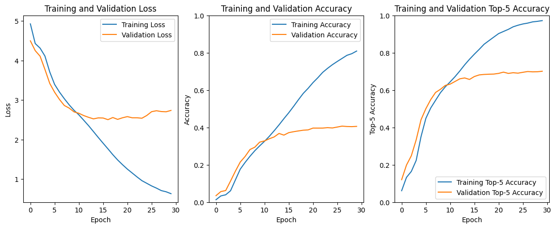

>> Validation 정확도는 40%이고, *Top-5 정확도는 70%를 기록함

*Top-5 정확도:
모델이 예측한 확률의 상위 5개 클래스 중에 정답 클래스가 하나라도 포함되어 있으면 맞은 것으로 처리

""" 📌 테스트 데이터 결과 확인 """
vit.evaluate(test_x, test_y)

>>> 313/313 [==============================] - 4s 13ms/step - loss: 2.7125 - accuracy: 0.4114 - top-5-accuracy: 0.7034
	[2.7125136852264404, 0.4113999903202057, 0.7034000158309937]

>> 테스트 정확도는 43%, Top-5 정확도는 72%를 기록함

---

스윈 트랜스포머

---

스윈 트랜스포머 실습