[이미지 처리 바이블] 교재 3장을 기반으로 작성되었습니다.
3.2 딥러닝을 활용한 이미지 처리
3.2.1 이미지 분류
분류를 위한 데이터 전처리
모듈 불러오기
import matplotlib.pyplot as plt
from tensorflow.keras.datasets import cifar10
from tensorflow.keras.models import Sequential
from tensorflow.keras.layers import Dense, Flatten
from tensorflow.keras.callbacks import ModelCheckpoint, EarlyStopping
데이터 불러오기
# CIFAR-10 데이터 세트를 불러옵니다.
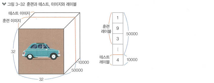
(train_images, train_labels), (test_images, test_labels) = cifar10.load_data()데이터 확인하기
# 데이터를 확인합니다.
print(train_images.shape, train_labels.shape)
print(test_images.shape, test_labels.shape)
>>> (50000, 32, 32, 3) (50000, 1)
(10000, 32, 32, 3) (10000, 1)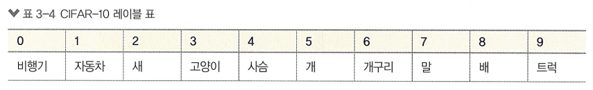
데이터 정규화
# 정규화된 이미지 데이터를 하나 확인합니다.
train_images[0]
>>> ndarray (32, 32, 3)# 확인을 위해 출력
plt.figure(figsize=(1, 1))
plt.imshow(train_images[32])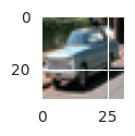
# 정규화를 위해 255로 나누어 줍니다.

train_images = train_images / 255.0
test_images = test_images / 255.0
# 정규화된 이미지 데이터 출력
train_images[0]>>> array([[[0.23137255, 0.24313725, 0.24705882],
[0.16862745, 0.18039216, 0.17647059],
[0.19607843, 0.18823529, 0.16862745],
...(중략)...
[0.84705882, 0.72156863, 0.54901961],
[0.59215686, 0.4627451 , 0.32941176],
[0.48235294, 0.36078431, 0.28235294]]])
# 모든 픽셀이 0에서 1사이의 값으로 정규화됨 --> 최적화 단계에서 더 빠르게 수렴하고 결과를 좋게 만듬데이터 분할(훈련, 검증)
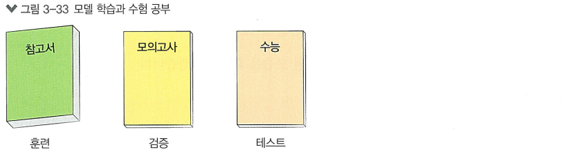
데이터는 훈련(train), 검증(validation), 테스트(test) 세트로 나눔
# 훈련 데이터셋과 검증 데이터셋으로 나누어 줍니다.

val_images = train_images[45000:]
val_labels = train_labels[45000:]

train_images = train_images[:45000]
train_labels = train_labels[:45000]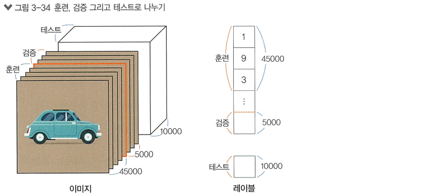
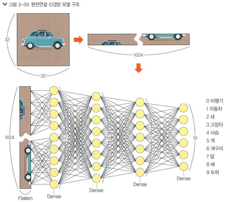
MLP를 활용한 이미지 분류
다층 퍼셉트론은 "모든 뉴런들끼리 결합"되어 있어 fully-connected neural network 라고도 부름
3개의 은닉층을 쌓은 다층 퍼셉트론 모델을 구현해볼 것임
# 모델을 생성합니다.
mlp_model = Sequential([
    Flatten(input_shape=(32, 32, 3)),	# 1.입력층
    Dense(512, activation='relu'),		# 2.은닉층
    Dense(256, activation='relu'),		# 2.은닉층
    Dense(128, activation='relu'),		# 2.은닉층
    Dense(10, activation='softmax')		# 3.출력층
])
1. 입력층
> Flatten 층을 사용하여 (32x32x3)의 3차원 이미지의 모든 픽셀 정보를 한 줄로 쫙 펴서
크기가 3,072인 1차원 벡터로 변환하고, 이를 밀집층에 연결함
2. 은닉층
> 신경망의 핵심적인 부분으로, 입력 데이터의 비선형 관계를 학습함
3. 출력층
> 신경망에서 최종적으로 나오는 결과 값을 표현하는 층
분류에선 각 클래스에 대한 확률을 출력, 회귀에선 연속적인 값을 출력
"출력층의 뉴런 개수는 우리가 예측하려는 레이블의 개수로 설정함"
# 모델의 구조를 확인합니다.
mlp_model.summary()
>>> Model: "sequential"
┏━━━━━━━━━━━━━━━━━━━━━━━━━━━━━━━━━━━━━━┳━━━━━━━━━━━━━━━━━━━━━━━━━━━━━┳━━━━━━━━━━━━━━━━━┓
┃ Layer (type) ┃ Output Shape ┃ Param # ┃
┡━━━━━━━━━━━━━━━━━━━━━━━━━━━━━━━━━━━━━━╇━━━━━━━━━━━━━━━━━━━━━━━━━━━━━╇━━━━━━━━━━━━━━━━━┩
│ flatten (Flatten) │ (None, 3072) │ 0 │
├──────────────────────────────────────┼─────────────────────────────┼─────────────────┤
│ dense (Dense) │ (None, 512) │ 1,573,376 │
├──────────────────────────────────────┼─────────────────────────────┼─────────────────┤
│ dense_1 (Dense) │ (None, 256) │ 131,328 │
├──────────────────────────────────────┼─────────────────────────────┼─────────────────┤
│ dense_2 (Dense) │ (None, 128) │ 32,896 │
├──────────────────────────────────────┼─────────────────────────────┼─────────────────┤
│ dense_3 (Dense) │ (None, 10) │ 1,290 │
└──────────────────────────────────────┴─────────────────────────────┴─────────────────┘
Total params: 1,738,890 (6.63 MB)
Trainable params: 1,738,890 (6.63 MB)
Non-trainable params: 0 (0.00 B)Layer (type) = 모델이 사용하는 층의 이름과 타입
Output Shape = 층의 출력 형태를 나타냄 (배치 사이즈, 출력 형태).
모델 학습 전엔 배치 사이즈를 알 수 없기 때문에 None으로 적힘
Param # = 층의 학습 매개변수 개수를 나타냄
모델 컴파일하기
# 모델을 컴파일합니다.
mlp_model.compile(optimizer='adam',							# 최적화 알고리즘 설정
                  loss='sparse_categorical_crossentropy',	# 손실 함수 설정
                  metrics=['accuracy'])						# 모델의 평가 방법 설정
모델 훈련하기
# 모델을 훈련합니다.
mlp_model.fit(train_images, train_labels, epochs=5, validation_data=(val_images, val_labels))
>>> Epoch 1/5
1407/1407 ━━━━━━━━━━━━━━━━━━━━ 9s 4ms/step - accuracy: 0.2646 - loss: 2.0126 - val_accuracy: 0.3544 - val_loss: 1.7919
Epoch 2/5
1407/1407 ━━━━━━━━━━━━━━━━━━━━ 6s 3ms/step - accuracy: 0.3832 - loss: 1.7241 - val_accuracy: 0.4104 - val_loss: 1.6439
Epoch 3/5
1407/1407 ━━━━━━━━━━━━━━━━━━━━ 4s 3ms/step - accuracy: 0.4129 - loss: 1.6310 - val_accuracy: 0.4270 - val_loss: 1.6039
Epoch 4/5
1407/1407 ━━━━━━━━━━━━━━━━━━━━ 5s 3ms/step - accuracy: 0.4397 - loss: 1.5578 - val_accuracy: 0.4438 - val_loss: 1.5901
Epoch 5/5
1407/1407 ━━━━━━━━━━━━━━━━━━━━ 4s 3ms/step - accuracy: 0.4539 - loss: 1.5135 - val_accuracy: 0.4512 - val_loss: 1.5468
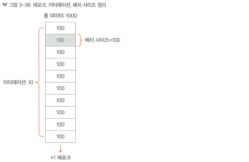
<keras.src.callbacks.history.History at 0x7c8fa54a7710>>> (미니 배치 경사하강법에서 하나의 배치에 해당하는 데이터의 개수를 의미)
batch_size를 따로 지정해주지 않아 기본 값인 32로 설정됨
45,000개의 데이터를 32개씩 묶어서 학습했고, 따라서 에포크마다 총 1,407번의 이터레이션이 이루어짐
5번째 에포크에서 검증용 데이터세트의 정확도는 약 45%를 기록함
총 데이터 수 = 1000, batch_size = 100 일땐, 한 번의 에포크를 돌기 위해선 10회의 이터레이션을 반복해야함
이터레이션은 '한 번의 에포크 학습을 위해 걸리는 배치 학습의 횟수'임
모델 평가하기
# 모델을 평가합니다.
mlp_model.evaluate(test_images, test_labels)
>>> 313/313 ━━━━━━━━━━━━━━━━━━━━ 1s 4ms/step - accuracy: 0.4506 - loss: 1.5365
[1.5445533990859985, 0.44290000200271606]> 약 45%의 정확도를 보임
> 이미지 처리에서 다층 퍼셉트론은 한계가 존재함
- 고차원 데이터 처리의 비효율성: 모든 노드가 fully-connected 되어 있기에 가중치 수가 급격히 증가함
- 공간적 구조 정보의 손실: 모든 픽셀값을 일렬로 펼치기에 이미지의 공간정보가 손실됨
- 스케일과 변형에 대한 민감성: MLP는 이미지 내 객체의 변화에 취약함. 민감하게 반응하여 다른 객체로 인식함
> 더 높은 성능/효율을 위해 이미지 처리에 강한 CNN을 활용해볼것임.
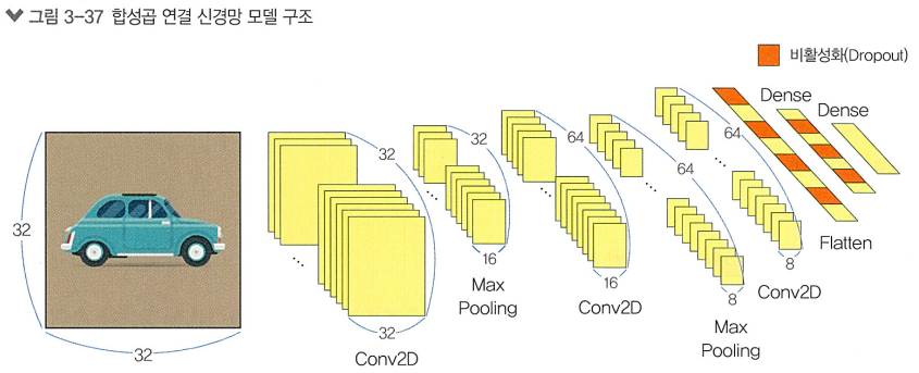
CNN을 활용한 이미지 분류
모델 생성하기
# 모듈 불러오기
from tensorflow.keras.layers import Conv2D, MaxPooling2D, Dropout

# 모델을 만듭니다.
cnn_model = Sequential([
    Conv2D(32, (3, 3), padding='same', activation='relu', input_shape=(32, 32, 3)),	# 1.합성곱 층
    MaxPooling2D((2, 2)),															# 2.풀링 층
    Conv2D(64, (3, 3), padding='same', activation='relu'),							# 1.합성곱 층
    MaxPooling2D((2, 2)),															# 2.풀링 층
    Conv2D(64, (3, 3), padding='same', activation='relu'),							# 1.합성곱 층
    Flatten(),	# Dense 층은 1차원 벡터만 받을 수 있으므로 3D 데이터를 일렬로 펴줌
    Dropout(0.3),																	# 3.드롭아웃 층
    Dense(64, activation='relu'),													# 4.밀집층
    Dropout(0.5),																	# 3.드롭아웃 층
    Dense(10, activation='softmax')													# 4.밀집층
    ])
1. 합성곱 층
> Conv2D 층의 첫번째 매개변수는 필터의 개수를 의미함 (32개)
두번째 매개변수는 필터의 사이즈를 의미함 (3x3)
패딩을 추가했고, ReLU 활성화함수 사용, 입력이미지의 사이즈를 명시함
2. 풀링 층
> MaxPooling2D 층은 풀링의 사이즈를 설정할 수 있는데, (2x2)로 설정했음
3. 드롭아웃 층
> Dropout(0,3) 기법을 적용하여,
학습 과정에서 무작위로 30%의 뉴런을 일시적으로 비활성화해서
네트워크 과적합을 방지함
4. 밀집층
> 첫번째 Dense층은 64개의 뉴런을 가지며 1차원으로 변환된 특징 맵의 뉴런 개수를 줄여주고,
두번째 Dense층은 10개의 뉴런을 가지며 10개의 클래스에 대한 확률을 출력해줌
# 모델의 구조를 확인합니다.
cnn_model.summary()
>>> Model: "sequential_1"
┏━━━━━━━━━━━━━━━━━━━━━━━━━━━━━━━━━━━━━━┳━━━━━━━━━━━━━━━━━━━━━━━━━━━━━┳━━━━━━━━━━━━━━━━━┓
┃ Layer (type) ┃ Output Shape ┃ Param # ┃
┡━━━━━━━━━━━━━━━━━━━━━━━━━━━━━━━━━━━━━━╇━━━━━━━━━━━━━━━━━━━━━━━━━━━━━╇━━━━━━━━━━━━━━━━━┩
│ conv2d (Conv2D) │ (None, 32, 32, 32) │ 896 │
├──────────────────────────────────────┼─────────────────────────────┼─────────────────┤
│ max_pooling2d (MaxPooling2D) │ (None, 16, 16, 32) │ 0 │
├──────────────────────────────────────┼─────────────────────────────┼─────────────────┤
│ conv2d_1 (Conv2D) │ (None, 16, 16, 64) │ 18,496 │
├──────────────────────────────────────┼─────────────────────────────┼─────────────────┤
│ max_pooling2d_1 (MaxPooling2D) │ (None, 8, 8, 64) │ 0 │
├──────────────────────────────────────┼─────────────────────────────┼─────────────────┤
│ conv2d_2 (Conv2D) │ (None, 8, 8, 64) │ 36,928 │
├──────────────────────────────────────┼─────────────────────────────┼─────────────────┤
│ flatten_1 (Flatten) │ (None, 4096) │ 0 │
├──────────────────────────────────────┼─────────────────────────────┼─────────────────┤
│ dropout (Dropout) │ (None, 4096) │ 0 │
├──────────────────────────────────────┼─────────────────────────────┼─────────────────┤
│ dense_4 (Dense) │ (None, 64) │ 262,208 │
├──────────────────────────────────────┼─────────────────────────────┼─────────────────┤
│ dropout_1 (Dropout) │ (None, 64) │ 0 │
├──────────────────────────────────────┼─────────────────────────────┼─────────────────┤
│ dense_5 (Dense) │ (None, 10) │ 650 │
└──────────────────────────────────────┴─────────────────────────────┴─────────────────┘
Total params: 319,178 (1.22 MB)
Trainable params: 319,178 (1.22 MB)
Non-trainable params: 0 (0.00 B)모델 컴파일하기
# 모델을 컴파일합니다. (MLP와 동일한 인수 사용)
cnn_model.compile(optimizer='adam',
                loss='sparse_categorical_crossentropy',
                metrics=['accuracy'])
콜백 정의하기
모델을 얼만큼 학습해야 과소/과대적합이 아닌 적절한 모델을 얻을 수 있는지 알기위해,
마지막 에포크 전에 가장 좋은 성능인 best model을 가져올 수 있게 하기 위해 콜백을 사용함
# EarlyStopping, ModelCheckpoint 콜백을 정의합니다.

from tensorflow.keras.callbacks import EarlyStopping, ModelCheckpoint

early_stopping = EarlyStopping(monitor='val_loss', patience=5)
save_best_only = ModelCheckpoint('best_cifar10_cnn_model.h5', save_best_only=True)
EarlyStopping 인수
- monitor: 어떤 값을 기준으로 삼을 것인지 정함 (val_loss를 사용하여 검증 손실을 기준으로 삼음)
- patience: 얼마나 기다릴 것인지 정함 (5번이상 검증 손실이 감소하지 않으면 학습 중단)ModelCheckPoint 인수
- filepath: 모델을 저장할 파일 경로를 지정 ('현재폴더에' 'best_cifar10_cnn_model.h5'라는 이름으로 저장)
- save_best_only: 가장 좋은 성능의 모델만 저장할 것인지 정함
모델 학습하기
# 모델을 학습시킵니다. (중간에 학습이 중단되는 것이 정상)
history = cnn_model.fit(train_images, train_labels, batch_size=512, epochs=100, validation_data=(val_images, val_labels), callbacks=[early_stopping, save_best_only])
>>> Epoch 1/100
88/88 ━━━━━━━━━━━━━━━━━━━━ 0s 49ms/step - accuracy: 0.2170 - loss: 2.1037WARNING:absl:You are saving your model as an HDF5 file via `model.save()` or `keras.saving.save_model(model)`. This file format is considered legacy. We recommend using instead the native Keras format, e.g. `model.save('my_model.keras')` or `keras.saving.save_model(model, 'my_model.keras')`.
88/88 ━━━━━━━━━━━━━━━━━━━━ 14s 83ms/step - accuracy: 0.2178 - loss: 2.1019 - val_accuracy: 0.4514 - val_loss: 1.5609
Epoch 2/100
87/88 ━━━━━━━━━━━━━━━━━━━━ 0s 16ms/step - accuracy: 0.4010 - loss: 1.6459WARNING:absl:You are saving your model as an HDF5 file via `model.save()` or `keras.saving.save_model(model)`. This file format is considered legacy. We recommend using instead the native Keras format, e.g. `model.save('my_model.keras')` or `keras.saving.save_model(model, 'my_model.keras')`.
88/88 ━━━━━━━━━━━━━━━━━━━━ 2s 19ms/step - accuracy: 0.4013 - loss: 1.6451 - val_accuracy: 0.5150 - val_loss: 1.3726
...(중략)...
Epoch 47/100
88/88 ━━━━━━━━━━━━━━━━━━━━ 3s 19ms/step - accuracy: 0.7862 - loss: 0.5999 - val_accuracy: 0.7700 - val_loss: 0.6895
Epoch 48/100
88/88 ━━━━━━━━━━━━━━━━━━━━ 2s 17ms/step - accuracy: 0.7884 - loss: 0.5881 - val_accuracy: 0.7756 - val_loss: 0.6873
>> 콜백에 따라 48번째 에포크에서 학습이 중단됨!
# 각 스텝의 학습 손실과 검증 손실을 그래프로 나타냅니다.
plt.plot(history.history['loss'], 'b--')
plt.plot(history.history['val_loss'], 'r--')
plt.xlabel('epoch')
plt.ylabel('loss')
plt.legend(['train loss', 'validation loss'])
plt.show()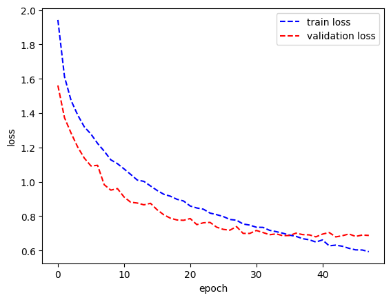
모델 평가하기
# 모델을 평가합니다.
cnn_model.evaluate(test_images, test_labels)
>>> 313/313 ━━━━━━━━━━━━━━━━━━━━ 2s 4ms/step - accuracy: 0.7687 - loss: 0.6937
[0.7016852498054504, 0.7649999856948853]평가 결과, MLP 모델의 45%보다 약 31% 정도 높은 76%의 정확도를 얻었음
예측 결과 시각화
"""예측 레이블 배열 생성"""
predicted_labels = cnn_model.predict(test_images)
predicted_labels.shape
>>> 313/313 ━━━━━━━━━━━━━━━━━━━━ 1s 3ms/step
(10000, 10)하나의 레이블에 대해 길이 10의 배열이 반환됨. (10개의 클래스에 대한 각각의 확률값)
아래와 같이 이 중 가장 큰 값을 가지는 인덱스를 뽑아내 예측 레이블로 사용하도록 함
"""각 배열의 최대 값의 색인을 뽑아내어 예측 레이블로 사용"""

import tensorflow as tf

predicted_labels = tf.argmax(predicted_labels, axis=1)
predicted_labels
>>> <tf.Tensor: shape=(10000,), dtype=int64, numpy=array([3, 8, 8, ..., 5, 1, 7])>"""레이블의 정수 값에 클래스 이름을 대응시켜 딕셔너리 생성"""
label_to_name = {
0: 'airplane', 1: 'automobile', 2: 'bird', 3: 'cat', 4: 'deer',
5: 'dog', 6: 'frog', 7: 'horse', 8: 'ship', 9: 'truck'
}"""test_images를 시각화하여 test_labels와 predicted_labels를 비교합니다.
test_labels와 predicted_labels가 다를 때, xlabel의 색깔을 빨강색으로 변경합니다."""
import matplotlib.pyplot as plt
plt.figure(figsize=(10, 10))
for i in range(16):
plt.subplot(4, 4, i+1)
plt.xticks([])
plt.yticks([])
plt.imshow(test_images[i], cmap=plt.cm.binary)
xlabel = f"{label_to_name[int(test_labels[i][0])]} ({label_to_name[int(predicted_labels[i])]})"
plt.xlabel(xlabel, color='red' if test_labels[i][0] != predicted_labels[i] else 'black')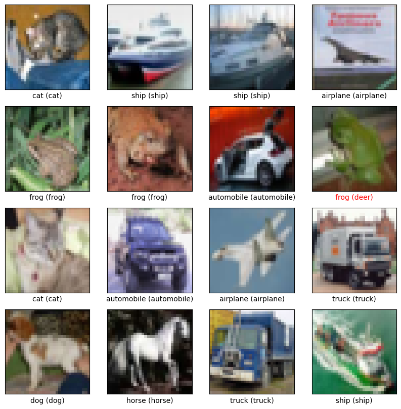
3.2.2 객체 인식
하르 캐스케이드
> 2001년에 소개된 객체 탐지 알고리즘
효과적인 특징 추출과 Adabooks 알고리즘을 사용해 작동
특징 추출
> 이미지의 픽셀은 그리드로 구성되어 있으며, 각 픽셀은 색상/강도 정보를 포함함
이런 픽셀 정보를 이용해 영역의 특징을 추출함
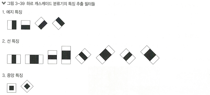
다양한 사이즈/모양의 하르 캐스케이드 특징을 사용해 이미지의 다양한 특성 포착
각 영역에서 픽셀 강도의 차이를 계산해 특징 값을 추출함
하르 캐스케이드 특징의 스케일과 위치
> 객체는 위치나 크기에 따라 다양하게 나타나므로 다양한 크기와 위치를 고려해 탐지해야 함
이를 위해 두 가지 스케일링 방식이 사용됨:
- 이미지 스케일링: 이미지를 여러 크기로 축소/확대해 객체를 탐지함.
- 특징 스케일링: 하르 특징 자체의 크기를 조절해 다양한 크기의 객체를 탐지함.
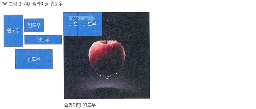
> 이미지 내의 다양한 위치에서 객체가 나타날 수 있기 때문에,
위치를 검출하는데 사용되는 방법론들은 아래와 같음
- 슬라이딩 윈도우: 이미지 전체를 횡단하며 하르 캐스케이드 특징을 추출해 객체를 탐지
- 스트라이드: 슬라이딩 윈도우를 얼마나 빠르게 이동시킬지 정하는 값
에이다부스트
하르 캐스케이드 특징을 사용해 이미지에서 특징을 추출한 후 이 특징들을 분류기에 입력으로 제공하는데, '단일 분류기'만 사용하는 것은 제한적이기에 '여러 개의 분류기'를 결합하여 성능을 올린 앙상블 기법
부스팅(Boosting)은 머신러닝의 앙상블 기법 중 하나로, 여러 개의 개별 모델을 결합해 하나의 Best 모델을 생성하는 방법이다. AdaBoost가 가장 널리 사용됨

Diagram of the AdaBoost Algorithm
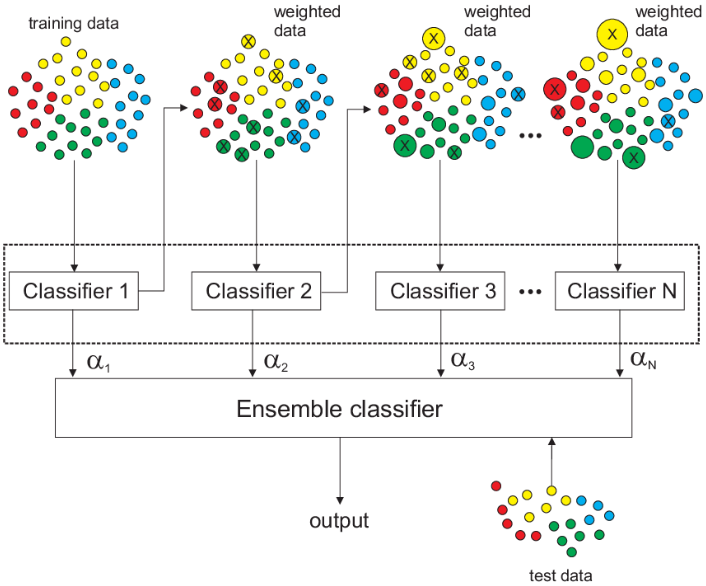
데이터 샘플과 가중치 초기화
Adaboost는 모든 학습 샘플에 동일한 가중치를 부여하며 시작함
>> (어떤 샘플이 알고리즘이 도움이 되는지 알 수 없기 때문)
- : 번째 샘플의 가중치
- : 전체 샘플의 수
반복적인 학습
약한 학습기(Weak learner)의 오차 계산
- : 약한 학습기의 가중치 오차
- : 번째 샘플에 대한 예측 오차 (맞으면 0, 틀리면 1)
학습기 가중치 수식
- : 학습기의 가중치
>> 학습기가 잘 작동할수록 (이 작을수록) 값이 커지는 원리
샘플 가중치 업데이트 수식
- : 번째 샘플의 실제 레이블
- : 번째 샘플에 대한 학습기의 예측 값
>> 학습기의 오류를 계산하고, 이를 기반으로 학습기에 가중치를 부여
>> 잘못 분류된 샘플의 가중치는 증가, 올바르게 분류된 샘플의 가중치는 감소
>> Adaboost는 여러개의 약한 학습기를 순차적으로 학습시키는데,
잘못 맞춘 샘플에 집중해야 약한 학습기들이 보완되기 때문
결합
모든 약한 학습기를 결합해 강한 학습기를 생성함
- : 최종 모델의 예측
- : 전체 학습기의 수
OpenCV를 활용한 하르 캐스케이드 구현 실습
import cv2
import matplotlib.pyplot as plt

!wget https://raw.githubusercontent.com/Lilcob/test_colab/main/three%20young%20man.jpg

# 이미지 로드
image_path = "/content/three young man.jpg"
image = cv2.imread(image_path)
gray = cv2.cvtColor(image, cv2.COLOR_BGR2GRAY)

# 하르 캐스케이드 로드 (사전 훈련된 하르 캐스케이드 XML 파일 포함)
face_cascade = cv2.CascadeClassifier(cv2.data.haarcascades + "haarcascade_frontalface_default.xml")

# 정면 얼굴 탐지
faces = face_cascade.detectMultiScale(gray, scaleFactor=1.1, minNeighbors=5, minSize=(30, 30))
print(faces)
>>> [[449 111 173 173]
[721 106 170 170]
[159 148 160 160]
[371 376 116 116]]# 탐지된 얼굴에 사각형 그리기
for (x, y, w, h) in faces:
cv2.rectangle(image, (x, y), (x+w, y+h), (255, 0, 0), 2)
# 결과 표시
plt.imshow(cv2.cvtColor(image, cv2.COLOR_BGR2RGB))
plt.axis('off') # 축 정보 숨기기
plt.show()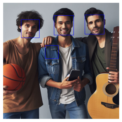
3.2.3 스타일 전이
스타일 전이란?
> 한 이미지의 스타일을 다른 이미지에 전이시키는 기술
ex) 내가 찍은 사진을 반 고흐의 그림 스타일로 변환
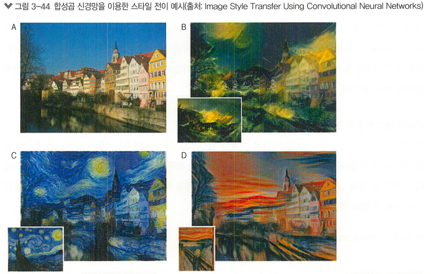
스타일 전이의 두 가지 핵심 개념:
- 콘텐츠 포현: 이미지의 구조, 형태, 객체 등 내용적인 요소
- 스타일 표현: 색상 조합, 붓질, 텍스처 등 느낌이나 방식
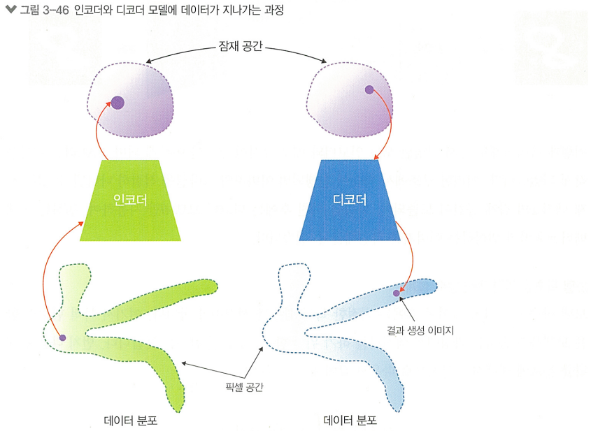
VAE를 활용한 잠재 벡터 추출
이미지 생성 모델의 구현 가능성
원하는 특징을 가진 이미지를 생성하는 모델을 만들고 싶다면, 특징 벡터를 입력으로 받아 원하는 특징을 결과 값으로 반환하는 모델 구조를 구상하게 됨.
> 여기서 특징을 표현하는 벡터를 잠재 벡터(Latent Vector)라고 부름
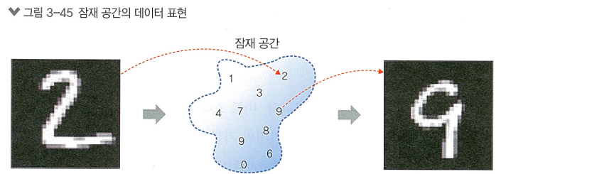
> 원하는 특징에 대한 이미지를 만들기 위해 가장 기본적이면서도 대표적인 모델로 VAE(Variational AutoEncoder)가 있음
VAE의 목적: "원하는 특징을 가진 이미지를 만들어낼 수 있는가?"
곱규칙에 의해
- : 잠재벡터
- : 를 받아 이미지를 만들어주는 디코더 모델
- : 모델 에 따른 확률 분포
- : 실제 생성하고 싶은 이미지 데이터 세트의 분포
전체 데이터 분포 X는 관측할 수 없기에 는 알 수 없고, 도 알기 알기어려움
>> 근사 기법 적용해서 해결해봄- : 원하는 이미지 를 만들기 위한 잠재 벡터 를 찾기위한 모델 (역추적모델) = 인코더
>> 를 하나 구성해주면, 우리가 원하는 이미지의 특성을 조절하여 이미지를 변화시킬 수 있을것
모델 의 결과값 잠재 벡터 는 매번 다르게 나타날 수 있음
> 이를 참조해서 잠재 벡터 를 랜덤 추출해내는 방식인 variational inference 사용- : 평균 , 표준편차 를 따르는 정규분포
이렇게 랜덤 추출된 벡터는 모델이 데이터의 특성을 더 잘 학습할 수 있게끔 도와줌
>> 모델이 더 일반화된 특성을 배우도록 강제하기 때문!
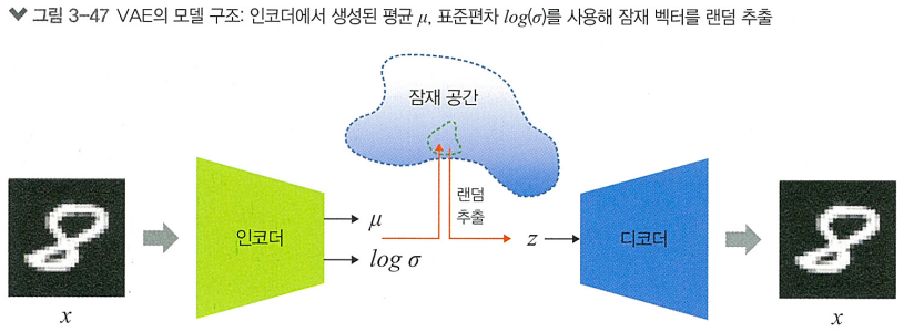
>> 결국 인코더를 지난 벡터 z의 잠재 공간이 도출되고, 변하는 잠재 벡터 z에 따라 도출되는 이미지는 변함
모델 학습을 위한 목적 함수 설계
(?)
텐서플로를 활용한 VAE 모델 구현 및 학습
from IPython import display

import glob
import imageio
import matplotlib.pyplot as plt
import numpy as np
import tensorflow as tf
import tensorflow_probability as tfp
import time

# ✅ 데이터 세트 준비
(train_images, _), (_, _) = tf.keras.datasets.mnist.load_data()

def preprocess_images(images):
    images = images.reshape((images.shape[0], 28, 28, 1)) / 255.
    return np.where(images > .5, 1.0, 0.0).astype('float32')

train_images = preprocess_images(train_images)

train_shuffle = 60000
batch_size = 128

train_dataset = (tf.data.Dataset.from_tensor_slices(train_images)
                 .shuffle(train_shuffle).batch(batch_size))

# ✅ 모델 구현
class VAE(tf.keras.Model):
    """Variational Autoencoder."""

    def __init__(self, latent_dim):
        super(VAE, self).__init__()
        self.latent_dim = latent_dim
        self.encoder = tf.keras.Sequential(
            [
                tf.keras.layers.InputLayer(input_shape=(28, 28, 1)),
                tf.keras.layers.Flatten(),
                tf.keras.layers.Dense(512, activation='relu'),
                tf.keras.layers.Dense(512, activation='relu'),
                # No activation
                tf.keras.layers.Dense(latent_dim + latent_dim),
            ]
        )

        self.decoder = tf.keras.Sequential(
            [
                tf.keras.layers.InputLayer(input_shape=(latent_dim,)),
                tf.keras.layers.Dense(512, activation='relu'),
                tf.keras.layers.Dense(512, activation='relu'),
                # No activation
                tf.keras.layers.Dense(28*28*1),
                tf.keras.layers.Reshape(target_shape=(28, 28, 1)),
            ]
        )

    @tf.function
    def sample(self, eps=None):
        if eps is None:
            eps = tf.random.normal(shape=(100, self.latent_dim))
        return self.decode(eps, apply_sigmoid=True)

    def encode(self, x):
        mean, logvar = tf.split(self.encoder(x), num_or_size_splits=2, axis=1)
        return mean, logvar

    def reparameterize(self, mean, logvar):
        eps = tf.random.normal(shape=mean.shape)
        return eps * tf.exp(logvar * .5) + mean

    def decode(self, z, apply_sigmoid=False):
        logits = self.decoder(z)
        if apply_sigmoid:
            probs = tf.sigmoid(logits)
            return probs
        return logits

# ✅ 손실 함수 정의, 최적화 기법
optimizer = tf.keras.optimizers.Adam(4e-4)  # Adam 사용


def log_normal_pdf(sample, mean, logvar, raxis=1):
    log2pi = tf.math.log(2. * np.pi)
    return tf.reduce_sum(
        -.5 * ((sample - mean) ** 2. * tf.exp(-logvar) + logvar + log2pi),
        axis=raxis)


def compute_loss(model, x):
    mean, logvar = model.encode(x)
    z = model.reparameterize(mean, logvar)
    x_logit = model.decode(z)
    cross_ent = tf.nn.sigmoid_cross_entropy_with_logits(logits=x_logit, labels=x)
    logpx_z = -tf.reduce_sum(cross_ent, axis=[1, 2, 3])
    logpz = log_normal_pdf(z, 0., 0.)
    logqz_x = log_normal_pdf(z, mean, logvar)
    return -tf.reduce_mean(logpx_z + logpz - logqz_x)

@tf.function
def train_step(model, x, optimizer):
    with tf.GradientTape() as tape:
        loss = compute_loss(model, x)
    gradients = tape.gradient(loss, model.trainable_variables)
    optimizer.apply_gradients(zip(gradients, model.trainable_variables))

# ✅ 모델 정의
epochs = 50
# 2차원 잠재 백터를 준비합니다.
latent_dim = 2
num_examples_to_generate = 25

# 생성(예측)을 위해 랜덤 벡터를 일정하게 유지하여
# 개선 사항을 더 쉽게 볼 수 있습니다.
random_vector_for_generation = tf.random.normal(
    shape=[num_examples_to_generate, latent_dim])
model = VAE(latent_dim)

# ✅ 학습 중 중간 진행 사항을 확인하기 위한 함수 정의
def generate_and_save_images(model, epoch, test_sample):
    mean, logvar = model.encode(test_sample)
    z = model.reparameterize(mean, logvar)
    predictions = model.sample(z)
    fig = plt.figure(figsize=(4, 4))

    for i in range(predictions.shape[0]):
        plt.subplot(5, 5, i + 1)
        plt.imshow(predictions[i, :, :, 0], cmap='gray')
        plt.axis('off')

    plt.savefig('image_at_epoch_{:04d}.png'.format(epoch))
    plt.show()

# 학습 중간에 확인할 데이터를 정해줍니다.
assert batch_size >= num_examples_to_generate
for test_batch in train_dataset.take(1):
    test_sample = test_batch[0:num_examples_to_generate, :, :, :]

# ✅ 모델 학습 진행
generate_and_save_images(model, 0, test_sample)

for epoch in range(1, epochs + 1):
    start_time = time.time()
    for train_x in train_dataset:
        train_step(model, train_x, optimizer)
    end_time = time.time()

    loss = tf.keras.metrics.Mean()
    for test_x in train_dataset:
        loss(compute_loss(model, test_x))
    elbo = -loss.result()
    display.clear_output(wait=False)
    print('Epoch: {}, ELBO: {}, time elapse for current epoch: {}'
          .format(epoch, elbo, end_time - start_time))
    generate_and_save_images(model, epoch, test_sample)
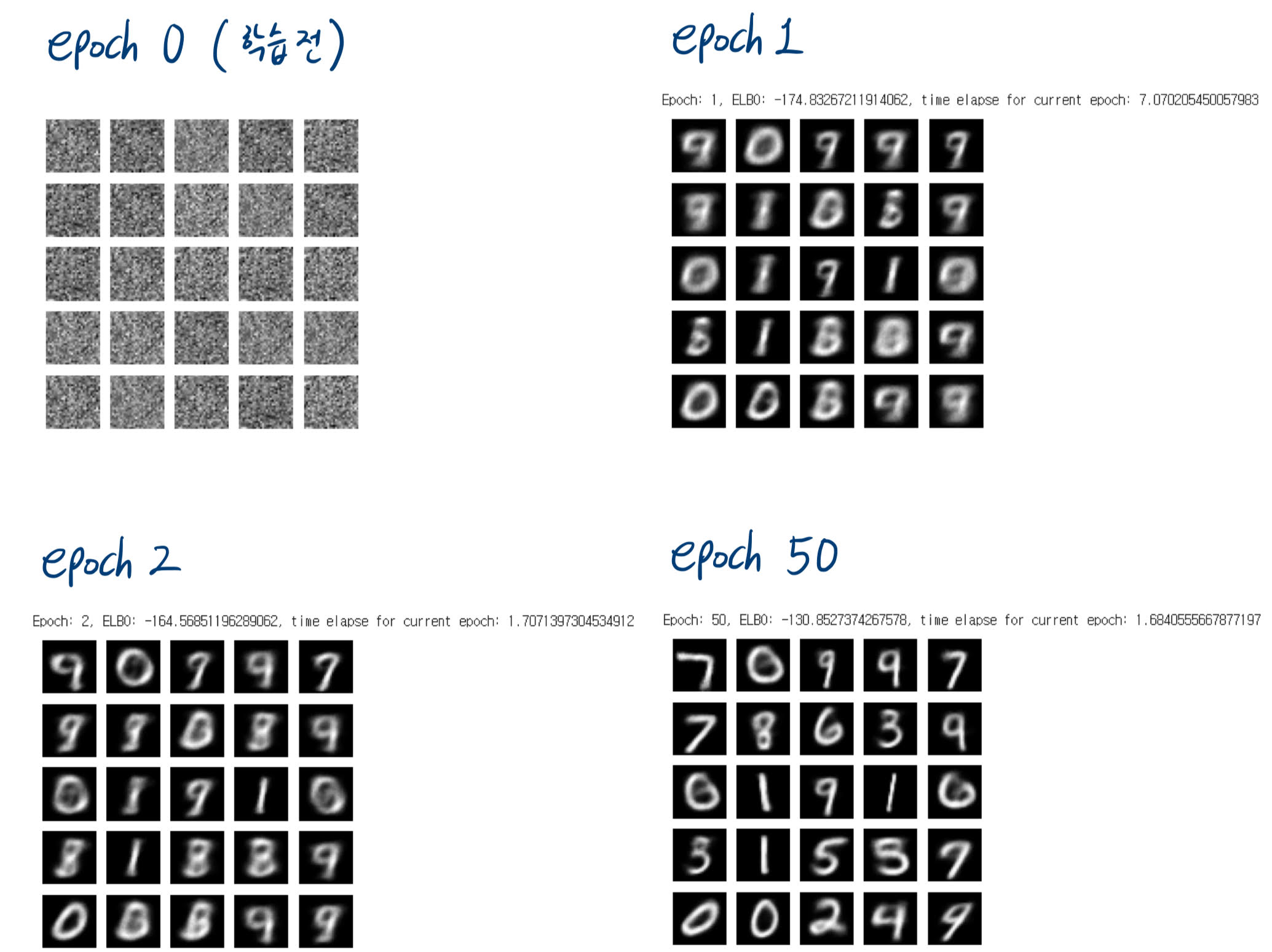
>> 학습 중간중간 어떻게 변하는지 확인 가능
# ✅ 2차원 잠재 공간의 벡터로부터 숫자가 어떻게 생성되는지 확인하기
def plot_latent_images(model, n, digit_size=28):
    """Plots n x n digit images decoded from the latent space."""

    norm = tfp.distributions.Normal(0, 1)
    grid_x = norm.quantile(np.linspace(0.05, 0.95, n))
    grid_y = norm.quantile(np.linspace(0.05, 0.95, n))
    image_width = digit_size*n
    image_height = image_width
    image = np.zeros((image_height, image_width))

    for i, yi in enumerate(grid_x):
        for j, xi in enumerate(grid_y):
            z = np.array([[xi, yi]])
            x_decoded = model.sample(z)
            digit = tf.reshape(x_decoded[0], (digit_size, digit_size))
            image[i * digit_size: (i + 1) * digit_size,
                  j * digit_size: (j + 1) * digit_size] = digit.numpy()

    plt.figure(figsize=(10, 10))
    plt.imshow(image, cmap='Greys_r')
    plt.axis('Off')
    plt.show()

plot_latent_images(model, 20)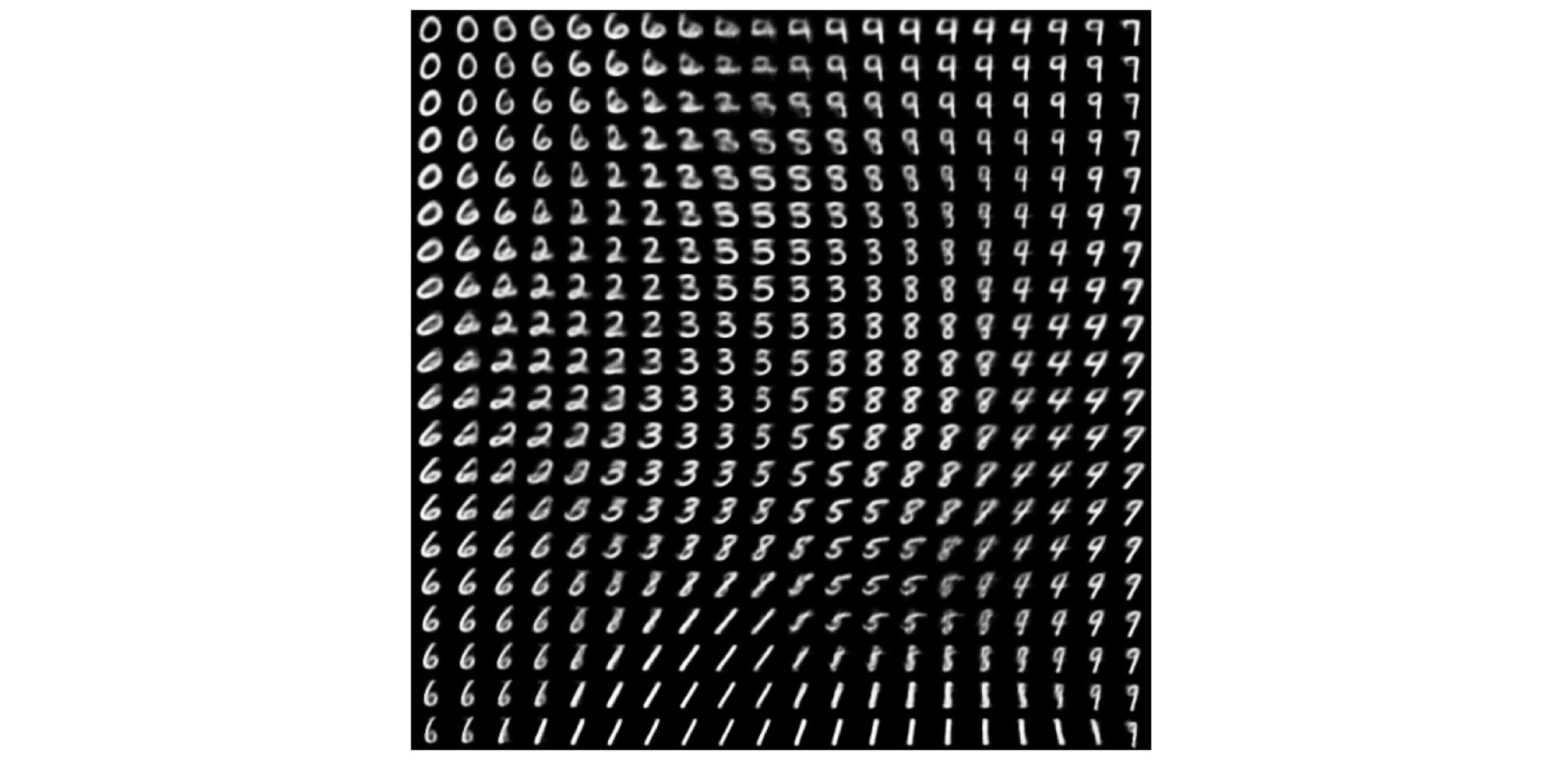
콘텐츠 표현과 스타일 표현의 추출
-
콘텐츠 표현: 이미지의 기본적인 구조와 형태를 표현
-
스타일 표현: 특징 맵을 통해 Gram Matrix(스타일 행렬)를 계산하고, 이를 통해 이미지의 텍스처와 패턴을 표현
스타일 전이 과정에서 손실 함수는 아래와 같이 정의함:
- : 전체 손실 함수
- : 콘텐츠 표현의 손실
- : 스타일 표현의 손실>> 값과 값을 조정해 이미지에 스타일이 적용되는 정도 조절
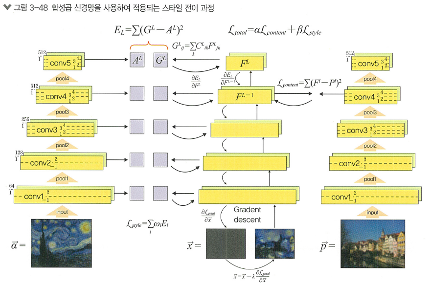
+) 그림 설명
이 그림은 스타일 전이를 합성곱 신경망(CNN)을 사용하여 구현하는 전체 흐름을 시각화한 것이다.
한 이미지의 내용(content) 과 다른 이미지의 스타일(style) 을 합쳐서 새로운 이미지를 만드는 과정을 보여준다.
✅ 등장인물 요약
| 기호 | 의미 |
|---|---|
| 콘텐츠 이미지 (예: 마을 사진) | |
| 스타일 이미지 (예: 고흐의 별이 빛나는 밤) | |
| 우리가 최종적으로 만들고 싶은 결과 이미지 | |
| 콘텐츠 손실 (내용이 얼마나 비슷한가) | |
| 스타일 손실 (화풍이 얼마나 비슷한가) | |
| 전체 손실 함수: 콘텐츠 + 스타일 가중합 |
🧠 전체 흐름 설명
1️⃣ 네트워크: 사전 학습된 CNN (VGG-19)
왼쪽, 오른쪽, 가운데에 똑같은 VGG가 등장한다.
- 오른쪽: 콘텐츠 이미지
- 왼쪽: 스타일 이미지
- 가운데: 결과 이미지
모두 VGG에 통과되어 feature map (특징맵) 을 뽑아낸다.
2️⃣ 콘텐츠 손실 계산
- → 특정 층 (
conv4_2)의 출력 = - → 같은 층의 출력 =
👉 콘텐츠 손실은 내용 유사도를 측정한다.
3️⃣ 스타일 손실 계산
- 스타일 이미지 와 결과 이미지 를 여러 층 (
conv1_1,conv2_1, ...)에 넣고, - 출력된 feature map들을 Gram 행렬로 변환한다.
👉 스타일 손실은 층 내부 피처 간 상관관계(GRAM) 유사도를 측정한다.
4️⃣ 전체 손실 함수
- : 콘텐츠 중요도
- : 스타일 중요도
5️⃣ 최적화 (Gradient Descent)
- 는 무작위 노이즈 이미지에서 시작한다.
- 이미지 자체를 최적화 변수로 보고, 손실을 줄이도록 반복 업데이트:
👉 즉, 이미지 자체가 역전파를 통해 계속 수정되는 구조다.
📌 최종 결과
- 콘텐츠 이미지의 구조를 가지면서
- 스타일 이미지의 느낌을 표현한
- 새로운 이미지 가 생성된다! 🎨
🔥 한 줄 요약
콘텐츠 이미지 + 스타일 이미지 → VGG 통과
→ 손실 함수 계산 → 결과 이미지 업데이트
→ 스타일을 입힌 콘텐츠 이미지 생성!